Download
1 / 12
120 likes | 234 Views
Modeling Ices in star-forming clouds: MCMC approach. Pavel Senin, following J acqueline Keane presentations August 11, 2006. Interstellar ices in star-forming regions:. Image from P.Ehrenfreund & A.G.G.M.Tielens. Iterative model.

E N D
Modeling Ices in star-forming clouds:MCMC approach Pavel Senin, following Jacqueline Keane presentations August 11, 2006.
Interstellar ices in star-forming regions: Image from P.Ehrenfreund & A.G.G.M.Tielens
Iterative model • Consists from equations that model physical processes that occur at the “surface” only or within the cloud only. • Sequential iterations run considerably long period of time.
MCMC Model • Proven to be surprisingly effective in many cases. • Surfaces, clouds and all processes an be combined in one model. • Can be parallelized and tweaked to run “fast”. • “Jump function” design demands for significant amount of work.
Bayesian Basics: • Bayes theorem: (posterior = standardized likelihood * prior) • Basically we need to specify the prior distribution (of molecules within ice clouds and at the “surface”)in order to apply Bayes theorem and get posterior distribution.
Markov Chains Basics: • A Markov chain is a process that corresponds to the “no memory” network: • To quantify the chain, we need to specify • Initial probability: P(X1) • Transition probability: P(Xt+1|Xt) ... ... Xn X1 X2 X3
What about Monte-Carlo? • Monte-Carlo integration: Remember:
MCMC Objectives: • The basic idea is to set up a long chain which starts at a pre-specified distribution taken from sample (or randomly generated biased samples) then traverses to the posterior distribution that sampled for results. • Distribution of Xn →π as n →, π is stationary distribution.
Metropolis-Hastings algorithm • Set an initial X1. • If the chain is currently at Xn = x, randomly propose a new state Xn+1 = y according to a proposal density q(y | x). • Accept the proposed jump with probability • If not accepted, Xn+1 = x.
“Hacking” Metropolis-Hastings algorithm • Our problem is multi-dimensional (various molecules, various transitions) – can be parallelized by updating each component separately or by partitions using specified M-H schemes for each. • A lot of tweaks already were found and published, maybe we will be able to apply some.
N chains = N samples + one burn-in for all Sampling strategies • “One thread” sampling: • Simultaneous runs: • Hybrid strategies? N samples from one chain burn-in period
Conclusion: • Assuming significant amount of work that already done for modeling physical processes “jump-function” design expected to be easier. • Model tuning should be easier to due to significant amount of data existed. • Both free MHPCC “PET” program and almost free student manpower allow cut cost of whole program to insignificant amount. – Worth to try.