Download
1 / 58
600 likes | 873 Views
Explore the fundamental concepts of units, relativistic kinematics, and cross section calculus in elementary particle physics lectures. Understand key principles such as natural units, decay width, and Lorentz transformations. Learn about units conversion, lifetime measurements, and 4-vector notation for relativistic kinematics.

E N D
ElementaryParticlePhysics Concepts Lectures2 & 3 Mark Thomson: Chapter 2 Chapter 3 David Griffiths: 6.3-6.5 Frank Linde, Nikhef, H044, f.linde@nikhef.nl, 020-5925140
Concepts(2&3): Units Relativistic kinematics cross section, lifetime, Feynman calculus toy model 2 3
Electromagnetism: Heaviside-Lorentz units q1 r12 units: q2 0allows to decouple unit of q from Time, Massand Lengthunits Coulomb: jullie! nu ikke … Thomson Griffiths unit of charge: qSI= 0 qHL= 04 qG Ampère:
Electromagnetism: Maxwell equations And for our applications: We experiment in vacuum so none of the complications of e.m. behavior in matter. And: often = 0 and j = 0 as well!
‘Natural’ units: h=c=1 e +e Units: Length[L] Time[T] Mass[M] Fundamental quantities:h 1.0566 1034Js(1 Js=1 kg m2/s) c 299792458 m/s (definition of meter) Simplify life by setting: c1 h1 • [L]=[T] • [M]=[L]=[T] Remaining freedom: pick as main unit Energy[E]=eV, keV, MeV, GeV, TeV, PeV, … Energy [E] GeV Momentum GeV/c Mass [M] GeV/c2 Time [T] h/GeV Lenght[L] hc/GeV
Common units in GeVx Relations between SI & natural units h = [Energy][Time] 1/h gets you from [s] to [GeV1] 1/(hc)2 gets you from [m2] to [GeV2] c = [Length]/[Time]
Units: lifetime – decay width Lifetime : [] = time s GeV1 Decay width 1/ : [ ] = 1/time s1 GeV conversion factor: 1/h 1.521024 (GeV s)1 = 2.1969811106 s 3.31018 GeV1 31010 eV
Units: lifetime – decay width be aware: often dominated by exp. resolution!
Units: cross section 1 barn U-nucleus Cross section : [] = area m2 GeV2 conversion factor: 1 nb1s1 ATLAS & CMS Luminosity: Ni: number of particles/bunch n: number of bunches/beam f: revolution frequency A: cross sectional area of beams L=fn LHCb ALICE LEP: 10+31 cm2s1= 10b1s1 100 pb1year1 “B-factory”: 10+33 cm2s1= 1 nb1s1 10 fb1year1 LHC: 10+34 cm2s1= 10 nb1s1 100 fb1year1 1 b = 1024 cm2 1 nb = 1033 cm2 1 pb = 1036 cm2 1 fb = 1039 cm2 typical “luminosities” L Ldt typical cross sections L = # of events Physics! (this course) Technology! (other course)
Lorentz transformation And: sorry for the many c’s still floating around here … S’ S v x’ x Co-moving coordinate systems: Einstein’s postulate: speed of light in vacuum always c y’ y Time dilatation: moving clocks tick slower! Time between events in rest frame S @ x=0 (0,0) & (,0) What measures S’ as time difference? Transform: (0,0) & (,…) Example:Cosmic-ray muons (210-6 s, m106 MeV): E=p=10 GeV vc, 100 travel typically 100c60 km
4-vector notation: conventions 4-vector: Invariant: same in frames S & S’ connected by Lorentz transformation: Introduce metric: Contra-variant 4-vector: Co-variant 4-vector: Generally for 4-vectors a and b: Note: ‘g= g’
Elegance/power of notation! S S’ For boosts contra-variant 4-vector: co-variant 4-vector: S’ S For rotationsupper/lower indices story remains the same i.e. same red expressions, numerically x & x transform identically - only spatial coordinates k=1, 2 & 3 enter the game
Derivatives: & 4-vectors Using: And chain rule: and this really makes a very elegant notation! Yields: transforms as a co-variant 4-vector! = = Hence: = = = corresponding contra-variant 4-vector:
* Lorentz transformations Lorentz-transformations: These matrices must obey: with invariant hence For infinitesimal transformations you find: Because: with or # of independent transformations: + Hence: 4x4–10=6 independent transformations: 3 rotations: around X-, Y- & Z-axis 3 ‘boosts’: along X-, Y- & Z-axis
* infinitesimal macroscopic from expression for ex … via Taylor expansion to cos & sin
* Lorentz transformations: rotations 0 1 2 3 S S’ 12 13 23 Lorentz Rotations around Z-axis (indices 1 & 2): 0 1 2 3 pick d as infinitesimal parameter: finite rotation around Z-axis yields: Similarly you find for the indices: 1 & 3 the rotations around the Y-axis • 2 & 3 the rotations around the X-axis
* cos, sin & cosh, sinh
* Lorentz transformations: boosts 0 1 2 3 01 02 03 Lorentz v Boosts along Z-axis (indices 0 & 3): S’ S 0 1 2 3 pick d as infinitesimal parameter: = finite boost along Z-axis yields: Relation between x0=ct, x3=z &x’0=ct’, x’3=z’: origin of S’ (z’=0) is seen by S at any time as: (t, vt) - - - and with cosh2sinh2=1, you get:
Velocity & Momentum 4-vectors u u’ S’ S x x’ Standard velocity definition: u x/t: For observer S: u = x /t For observer S’: u’= x’/t’ Lorentz transformation links u and u’: • u (and u’) not 4-vectors! • (not surprising: division of vector components …) 2nd attempt to define a velocity: use proper time =t/ or: d =dt/ 4-velocity: (hard to imagine nicer invariant) 4-momentum: • why p0E/c? • For particles with mass=0:
2-body decay: A B+C mB mA mC 2-body decay in c.m. frame Before decay: After decay: With: Example: -decay You get: m 140 MeV m 106 MeV E
Example particle decay: -decay ½m53 MeV m 106 MeV me 0.511 MeV Ee 53 MeV >2 particles
Threshold energy: anti-proton discovery B EA Threshold energy in Lab. Lab.: Lab. 1 2 c.m.: c.m. 3 4 (assumed mA=mB …) Threshold energy in c.m. frame: all particles produced at rest! energy in c.m. frame: c.m. Example: anti-proton Use this minimum energy (M) in the c.m. to calculate threshold energy in Lab.: p+p p+p+p+p 6.4 GeV
Bevatron: 6.5 billionelectron volts anti-proton annihilation
Mandelstam variables I: s, t & u D C lab cm B A A B D Lab-frame C c.m. frame E.g. in the lab. frame: EAlab & lab E.g. in the c.m. frame: EAcm & cm Useful Lorentz-invariant variables: For which you can easily prove: 4 4 3 3 12 8 5 2 rotations masses boosts momentum conservation 16 A + B C + D process characterized by 2 parameters cm lab EA EA
Mandelstam variables II: s, t & u Useful expressions in terms of s, t & u: Lab. frame: & beam energy, EA: c.m. frame: & total energy in c.m.: beam energy, EA: For A + A A + A, in the c.m. frame: = 4E2 (also if all m<< E) 2E2 2E2
Mandelstam variables III: s, t & u ‘s-channel’ ‘t-channel’ ‘u-channel’ Remark: p1, p2, p3 & p4 in these figures are the physical 4-momenta, arrows just flag particles (forward in time) and anti-particles (backward in time) And: direction of q you can pick, expressions for s, t & u do not depend on q-direction s (p1+p2)2=q2 t (p1-p3)2=q2 u (p1-p4)2=q2
ElementaryParticlePhysics Concepts Lectures 2 & 3 Mark Thomson: Chapter 2 Chapter 3 David Griffiths: 6.3-6.5 Frank Linde, Nikhef, H044, f.linde@nikhef.nl, 020-5925140
Exercise sessions Wednesdays 13:00-15:00 SP G3.13 SP G2.04 Fridays 09:00-11:00 SP A1.11 SP A1.14
Lifetime & Decay width mB mC mA c.m. frame Particle decay mathematics ( is decay width): particles # particles particles start decay: Lifetime ( ) decay-width ( ) connection: decays With multiple decay channels: partial decay-widths: i branching fraction: and = 1/tot Branching fractions: i/tot
Lifetime & Decay width l W+ l+
A+B C+D cross section Several factors playing a role: physics & ‘administration’: 1. Physics: transition probability Wfi(most of this course) probability for initial state ‘i’ to become final state ‘f’ units: [Wfi] = 1/(time volume) target 2a. Administration: flux i.e. beam- & target densities beam intensity: # of particles / (area time) target intensity: # of particles / (volume) units: [Flux] = 1/(area time volume) beam 2b. Administration: ’density’ of states ‘f’: phase space N=2 (or N for N particles) what really counts is the number density offinal states with more or less same properties i.e. 2 is just a weight/number (dimensionless) Cross section for A+B C+D becomes: [] = area Caveat: dimensions referred to don't account for wave function normalisations (later)
Example: cross section solid sphere b R Scattering upon a solidsphere (very simple, stupid geometry …) Geometry: Differential cross section: Total cross section: as it should be of course!
Intermezzo: Dirac - ‘function’ Definition of the Dirac -function: Fourier transforms: Take And therefore: examples:
Fermi’s ‘golden rule’ classical ‘Standard’ non-relativistic QM: complete set of statesnfor non-perturbed system forperturbed system express using n: solve iteratively for coefficients a(t) i.e. solve af(t) while assuming all coefficients ak, except the ith, to be 0: hence (f i): transition amplitude Tfi (f i): andfor a time independent perturbation (f i): with:
Fermi’s ‘golden rule’ classical Does |Tfi|2 represent the probability of an i f transition? no! Better ansatz: use |Tfi|2/T as i f transition probability per unit time: note: T-divergence no surprise: V(x) lasts forever! in real life: you control specific state with Ei nature picks any state with Ef sum over states with Ef introduce: # states with energy E: Fermi’s golden rule:
Relativistic expressions A+B C+D Relativistic free particlestates: plane waves transition amplitude alsobecomessimplesincethephysics part onlyinvolvesthe 4-momenta of in- & out-goingparticlepA, pB, pC& pD.Allhidden in Mfornow givesforthetransitionprobability: transition amplitude scaled per unit time & unit volume: note: T,V-divergence no surprise: plane waves: last forever & are everywhere! 4-momentum conservation!
Relativistic expressions A+B C+D N-particle phase-space: We will later show theparticledensity of tobe: L L Tocalculate we put everything in a cubewithperiodicboundaryconditions : L L L = V L particles/box 2E 2EV 1 E E Incidently: With # particles E, younicelymaintain consistent picture whenboostingbetween frames! v L L L L/
Relativistic expressions A+B C+D N-particle phase-space: Periodic boundary conditions: and similarly for y & z L L L spacing allowed momentum states is 2/L for px, py & pz density of states: L
Relativistic expressions A+B C+D N-particle phase-space: We will later show theparticledensity of tobe: L L Tocalculate we put everything in a cubewithperiodicboundaryconditions : L L L = V L particles/box 2E 2EV 1 1 particle/box: density of states in momentum space (periodicboundarayconditions): 2E particle/box:
Relativistic expressions A+B C+D Flux factor: v beam target 2EA/V 2EB/V remark on ‘volumes’: picture suggests different V for beam & target. not needed, but if you do: cancels against the N-dependent V terms in Wfi
Relativistic expressions A+B C+D Transition amplitude scaled by TV: = (1/V4) N-particle phase-space: Flux factor:
Relativistic expressions A+B C+D D C 1 1 C D c.m. frame Lab. frame Invariant form for A+B flux factor 4-momenta: p1=(E,p) & p2=(m2,0) 4-momenta: p1=(E1,+p) & p2=(E2,p) 2 2
Relativistic expressions A+B C+D Explicitly Lorentz invariant forms matrix element Lorentz invariant (later) (E,p)conservation Lorentz invariant phase space Lorentz invariant flux Lorentz invariant because:
Relativistic expressions A+B C+D Useful expressions for 2-particle phase-space Simplify 2-particle phase from 6 2 variables using the -function 1. Integrate over the 3-momentum of p4: E4 not an independent variable! & 2. With spherical coordinates d3p3=|p3|2d dp3 for p3: the dp3 integration is less trivial than it appears, but can be done using the -function paying attention to the p3 dependence hidden in its argument
Continue integration 3 1 2 c.m. frame 4 use: E2=p2+m2 3. In c.m. frame: define E=E1+E2 & E’=E3+E4 to find: to perform the integration over dp3=dp: remark: you can also do integration using:
Generic expressions for A+B C+D& A C+D C scattering A B D decay C A D A + B C + D cross section A C + D decay these expressions we will use repeatedly throughout this class
Example: A+B C+D scattering C A B c.m. frame D phase space: 2 = = check this! flux: cross section: question: units of ?