Download
1 / 26
260 likes | 466 Views
CSIM Simulation. ( or everything you want to know about CSIM but were afraid to ask). John C.S. Lui. Why we want to simulate?. Tradeoff between analytical modeling and system implementation Can relax the “restrictive” assumption in analytical modeling To “confirm” our analytical modeling.

E N D
CSIM Simulation (or everything you want to know about CSIM but were afraid to ask) John C.S. Lui
Why we want to simulate? • Tradeoff between analytical modeling and system implementation • Can relax the “restrictive” assumption in analytical modeling • To “confirm” our analytical modeling
Issues • What items need to be abstracted away, what cannot be abstracted away? • What are the performance measures I want? • How long do I need to run? What are the confidence intervals? • What is the run time of my simulation?
CSIM • Process-oriented, discrete event simulation. • Based on C or C++ • Easy to learn, takes moderate time to master. • If you know the concept of “processes”, then it will be EASY to learn CSIM in 30 mins.
Outline • CSIM: M/M/1 • CSIM: M/M/K • CSIM: Two servers with JSQ policy • CSIM: Fork-Join Queue • CSIM: Markov Chain Simulation • CSIM: Generating Synthetic Trace files
M/M/1 • Arrival process is Poisson, or the interarrival time is exponentially distributed. • Service time of a job is exponentially distributed. • TWO types of event: arrival, departure.
// C++/CSIM Model of M/M/1 queue // file: ex1cpp.cpp #include "cpp.h" // class definitions #define NARS 5000 // number of arrivals to simulate #define IAR_TM 2.0 // specify average interarrival time #define SRV_TM 1.0 // specify average service time event done("done"); // the event named done facility f("facility"); // the facility named f table tbl("resp tms"); // table of response times qhistogram qtbl("num in sys", 10l); // qhistogram of number in system int cnt; // count of remaining processe void customer(); extern "C" void sim(int, char **); void sim(int argc, char *argv[]) { set_model_name("M/M/1 Queue"); create("sim"); cnt = NARS; for(int i = 1; i <= NARS; i++) { hold(expntl(IAR_TM)); // interarrival interval customer(); // generate next customer } done.wait(); // wait for last customer to depart theory(); mdlstat(); // model statistics } void customer() // arriving customer { float t1; create("cust"); t1 = clock; // record start time qtbl.note_entry(); // note arrival f.reserve(); // reserve facility hold(expntl(SRV_TM)); // service interval f.release(); // release facility tbl.record(clock - t1); // record response time qtbl.note_exit(); // note departure if(--cnt == 0) done.set(); // if last customer, set done }
OUTPUT • Let us look at the output file, mm1.out, of the program ex1cpp.cpp • The “M/M/1” is our model name. • It displayed the “simulation time” • It displayed the “statistics” of facility “f”, table “resp tms” and qtable “QTABLE”. As well as the resource used. • Let us take a closer look of the output file, mm1.out, and see how we get performance measures.
Important concept about CSIM • CSIM has “passive” objects and “active” objects. • Passive object: facility, table, event, messages….etc • Active object: Customer. In other words, you CODE UP THE DYNAMICS • Differentiate “CPU time” and “simulation time”. • Dynamic object consumes CPU time, but it takes ZEROsimulation time UNLESS it executes statements like “hold”, “wait”, “reserve”, “release”….etc • Dynamic object (or a process) will GIVE UP the CPU resource to other “ready” process when it executes statements like “hold”, “wait”, “reserve”, “release”…etc.
Understanding the dynamics of CSIM • Let us look at the trace file, mm1_trace.out, of the previous program. • To limit the size of the trace file, set NARS to 20 • To turn on the trace, run the program like % a.out -T > mm1_trace.out • IF YOU UNDERSTAND THE TRACE, YOU UNDERSTAND THE PROCESS CONCEPT OF CSIM.
Trace File of M/M/1: mm1_trace.out • The first process, “sim”. • It generates a random # based on exp distribution. It “holds” (or sleep) for that amount of time (time is 1.332). • Since there is only ONE process (which is sim) in the CSIM kernel, so the simulation jumps to time t=1.332. • For the simulation time t=1.332, sim still has the CPU resource, it calls a function customer(). • The first statement of a function is “create”, which changes the function to a process. The thread of control goes back to the CSIM kernel. • There are two processes in the system, “sim” and “cust”, since sim DIDN’T give up its thread of control, the CSIM kernel gives the CPU to “sim”.
“sim” generates another random number based on exponential distribution, and “hold” (or sleep) at time t=1.332 and sleep for 3.477. Therefore, “sim” should wake up at t=4.809. • At simulation time t=1.332, thread of control goes back to csim kernel. Since there is only one “active” process, which is “cust”, that process has the CPU. • Process “cust” enters the empty facility and “hold” (or occupy the resource f) for some random time (generated by exp. distribution) of 1.176. This process should wait up at time 2.507. • Thread of control returns to CSIM kernel. Since at simulation time t=1.332, there is no more active process, kernel jumps to time=2.507, and gives the CPU to cust. • “cust” releases the resource and terminates.
Thread of control returns to CSIM kernel. At t=2.507, there is no more active process. So it jumps to the nearest time in which the system will have an active process, that is t=4.809. • At t=4.809, the only active process is “sim”. So sim has the CPU resource. • “sim” wakes up at t=4.809, calls the “customer” function. • Question: under what condition the system is stable?
Another way to look at the M/M/1 simulation • One process for traffic generation • Each job (or customer) as a process. • Have a “master” to control coordination. • Let us look at mm1_v2.cpp • Question: under what condition the system is stable?
Simple variation: M/M/K • Arrival is a Poisson process (or the interarrival time is exponentially distributed) with rate • The service rate of each server is exponentially distributed • Single queue, but with K servers. • CSIM provides many queueing functionalities. • Let us look at mmk.cpp and mmk.out • Question: under what situation the system is stable?
Two Servers with JSQ Policy • The system has two “independent” servers (e.g., with individual queue) • Arrival is Poisson • Service rate is exponential • Customer will choose the server with the “shorter” queue. • Let us look at shorter_queue.cpp and shorter_queue.out • Question: under what situation the system is stable?
Fork-Join Queueing System • Assume two independent servers • Job arrival rate is Poisson • Upon arrival, a job is splitted into two tasks, each join different queue • A job is completed when BOTH tasks are done (therefore, need synchronization) • Let us look at fork_join.cpp and fork_join.out • Question: under what situation the system is stable?
Other functionalities of CSIM • Facilities • Reserving a Facility with a Time-out: f.timed_reserved(10.0), …etc • hanging the Service Discipline: f.service(prc_shr), …etc • load dependent service rate: f.loaddep(rate, 10); • Inspector Methods: • f.qlength(): determine # of process waiting • f.completions(): number of completions so far • f.qlen(): mean queue length • f.tput(): mean throughput rate • Events • Waiting with a time-out: e.timed_wait(3.0); • Queueing for an event to occur: e.queue(); • Inspector Methods: • e.wait_cnt(): # of processes waiting for the event e. • e.state(): state of the event, either occurred or not occurred. • e.wait_length(): average wait queue length
Random number generation • Uniform(double min, double max); • Exponential(double mean); • Gamma (double mean, double stddev); • Hyperx( double mean, double var); • Zipf, Parteo, heavy tail distributions. • Single random number stream vs. multiple random number streams. • Tables: storing statistics • Qtable: to create historgram • Storages, Buffers, Mailboxes…etc • Other interesting features • Turn on/off the trace at any point in the program • Alter priority for processes • Managing queues • Confidence interval • Manipulating queued processes within a facility • Finite buffer to model communication network
Simulation of Markov Chain • Let us consider a Markov Chain for M/M/1 • For this MC, it has two events, arrival and departure (only when the number of jobs is greater than 0) • Paradigm: • For a given state, generate events • Determine which “type” of event • Determine the next state • Record state (for your performance measures) • Repeat • Program: mm1_mc.cpp
time M/M/1 via Markov Chain • Program: mm1_mc.cpp • Performance measures: average # of customers, average response time. N(t)
time M/M/1 via Markov Chain: state probability • Program: mm1_mc_prob.cpp • Let us consider the first few state probabilities. P[0] to P[4] and the rest is in P[5]. • Steady state probability: N(t) K
M/M/1 via Markov Chain: PASTA • PASTA: Poisson arrivals see time average • The previous state probability was an estimate for time average, let us see PASTA • Program: mm1_mc_pasta.cpp N(t) K n (or number of arrivals)
Generating Synthetic Trace File • Two classes of traffic: A and B • Interarrival time of class A (B) is exponential with mean being 10.0 (20.0) • For a particular class A (B) flow, the number of generated packets is uniformly distributed with inter-packet spacing exponentially distributed with mean being 2.0 (1.0) • We want to generate traffic for some duration T. • Program: tracefile.cpp
Conclusion • Simulation can help you • Build a better model • Validate your model • Takes time to debug (e.g., via tracing) • Needs to worry about transient errors, stability,…etc. • Yet, csim is a very powerful tool. You need to spend time reading the manual (which is well-written) to appreciate the power of this tool.