Download

1 / 22
230 likes | 253 Views
Simulation. Objective: To study and understand complex systems. A system is a collection of items from a circumscribed sector of reality that is the object of study. A model is an abstraction (description) of a system.

E N D
Simulation • Objective: To study and understand complex systems. • A system is a collection of items from a circumscribed sector of reality that is the object of study. • A modelis an abstraction (description) of a system. • Computer simulation is the process of designing a logical (mathematical) model of a real system and experimenting with this model via a computer to understand and predict its behavior. • Variance in the system is represented by probability distributions. • We repeatedly sample from these distributions to generate outcomes. (This process is nick named Monte Carlo simulation.)
Fun at Monaco’s Casinos… The mathematics behind Monte Carlo came out of the Manhattan Project to build the atomic bomb during World War II. The work is largely credited to Stanislaw Ulam, an Austrian-born mathematician, along with computer pioneer John von Neumann. The simulations offered a way of arriving at approximate solutions to troubling problems associated with random neutron diffusion in nuclear material. Ulam named the method ''Monte Carlo'' after a relative fond of sneaking off to Monaco's casinos.
Methods of Risk Analysis • Best/worst – case analysis • plug in the most optimistic/pessimistic values for each of the uncertain cells. • Easy but results in only two extreme data points! • What-if analysis • Plug in different values for the uncertain cells and see what happens • Appears easy (with spreadsheets) but unorganized and unscientific approach, also may require 100s of scenarios tested • Simulation • A systematic and unbiased approach to modeling and experimenting with a system.
Model Input Output Random Variables & Risk • A random variable is any variable whose value cannot be predicted or set with certainty. • Future interest rates • The number of customer arriving at a restaurant between 6-7 p.m. • The number of air force pilots leaving the service • The profit margin • Generally the value of one or more of the “independent”(input) variables is unknown or uncertain (hence making them random variables) • Consequently, the value of the dependent (output) variable(s) will be uncertain, therefore making the output(s) random variables • The uncertainty in the outcomes represents the riskin the decision making process.
Random Number Generators • Need RNs to simulate randomly occurring events, outcomes, etc. • All spreadsheets (and compilers and …) include a function for creating uniformly distributed random numbers between 0.0 and 1.0. • Simulate the coin toss • Simulate interest rate for the next quarter given: • P(rate cut) = 0.12, P(rate hike) = 0.55, and P(no change) = 0.33 • The “trick” used to generate random numbers for any given distribution is called the inverse transformation method. • All simulation add-ins like Analytic Solver Platform (Crystal Ball, @Risk, etc.)provide the most commonly used random number generators and a whole lot more…
Examples • Coin-toss example. • Hungry dawg example – basicvs. advanced approach. • Basic approach: uses averages (static), not distributions • Advanced approach: uses distributions; • From historical data, we found that the change in the number of covered employees each month is uniformly distributed between a 3% decrease and a 7% increase • The average claim per employee follows a normal distribution with mean increasing by 1% per month and a standard deviation of $3 • We can simulate using: • Data Tables, Descriptive Stats, etc. However, • Unnecessary when a tool like Analytic Solver or Crystal Ball available • Mont Carlo simulation using Analytic Solver Platform
Hungry Dawg Example • How much money should the Co. accrue to pay for the heath care claims? • For advanced approach, historical data analysis show that: • # of employees vary Uniformly between 3% decrease to 7% increase • U[-0.03, 0.07] (#of emp. of previous month)xU[0.97, 1.07] • Monthly claims vary Normally with the mean increasing by 1% and the std. dev. is $3 (regardless of the mean) • Month 1 N[250x1.01, 3] or N[252.50, 3] • Month 2 N[252.50x1.01, 3] or N[250x1.012, 3] • Month t N[250x1.01t, 3]
Piedmont (Commuter) Airlines • Facts: $150/ticket; $325/bump cost; 19 seats • Random variables: • No show probability 10% • Demand for seats: 14 3%, 15 5%, …, 25 2% • Business model implied, develop the profit function (step by step) • Suggestion: think of a couple of scenarios: • (Sample) decision: sell up to 20 tickets • Demand • No. show/no show • Revenue • Cost • Profit
Problem “Lynn Price…” • Age 30; invests $3,000/year in a fund with ROI Normal[12.5%, 2%] • How much $ will she have at the end of year at age 60?
Dr. Sarah Benson Dr. Sarah Benson is an ophthalmologist who, in addition to prescribing glasses and contact lenses, performs optical laser surgery to correct nearsightedness. This surgery is fairly easy and inexpensive to perform. Thus, it represents a potential gold mine for her practice. To inform the public about this procedure, Dr. Benson advertises in the local paper and holds information sessions in her office one night a week at which she shows a videotape about the procedure and answers any questions that potential patients might have. The room where these meetings are held can seat ten people, and reservations are required. The number of people attending each session varies from week to week. Dr. Benson cancels the meeting if two or fewer people have made reservations. Using data from the previous year, Dr. Benson determined that the distribution of reservations is as follows: Using data from the past year, Dr. Benson determined that each person who attends an information session has a 0.25 probability of electing to have the surgery. Of those who do not, most cite the cost of the procedure $2,000 as their major concern.
Dr. Sarah Benson - questions On average, how much revenue does Dr. Bensons practice in laser surgery generate each week? ( Use 5000 replications.) On average, how much revenue would the laser surgery generate each week if Dr. Benson did not cancel sessions with two or fewer reservations? Dr. Benson believes that 40% of the people attending the information sessions would have the surgery if she reduced the price to $ 1,500. Under this scenario, how much revenue could Dr. Benson expect to realize per week from laser surgery?
Ski Apparel Problem The owner of a ski apparel store in Winter Park, CO, must decide in July how many ski jackets to order for the following ski season. Each ski jacket costs $ 54 each and can be sold during the ski season for $145. Any unsold jackets at the end of the season are sold for $45. The demand for jackets is expected to follow a Poisson distribution with a average rate of 80. The store owner can order jackets in lot sizes of 10 units. How many jackets should the store owner order if she wants to maximize her expected profit? What are the best- case and worst- case outcomes the owner might face for this product if she implements your suggestion? How likely is it that the store owner will make at least $ 7,000 if she implements your suggestion? How likely is it that the store owner will make between $ 6,000 to $ 7,000 if she implements your suggestion? Take a few minutes to develop a simulation model Determine: facts; random variables; business model/logic flow…
Problem “Ski apparel….” Take a few minutes to develop a simulation model Facts; random variables; business model/logic flow…
The Uncertainty of Sampling • The replications of our model represent a sample from the (infinite) population of all possible replications. • As the sample size (# of replications) increases, the sample statistics converge to the true population values. • We can also construct confidence intervals for a number of statistics for:
Acme Equipment Co. Acme Equipment Company is considering the development of a new machine that would be marketed to tire manufacturers. Research and development costs for the project are expected to be about $ 4 million but could vary between $ 3 and $ 6 million. The market life for the product is estimated to be 3 to 8 years with all intervening possibilities being equally likely. The company thinks it will sell 250 units per year, but acknowledges that this figure could be as low as 50 or as high as 350. The company will sell the machine for about $ 23,000. Finally, the cost of manufacturing the machine is expected to be $ 14,000 but could be as low as $ 12,000 or as high as $ 18,000. The company’s cost of capital is 15%. Use appropriate RNGs to create a spreadsheet to calculate the possible net present values (NPVs) that could result from taking on this project. Replicate the model 5000 times. What is the expected NPV for this project? What is the probability of this project generating a positive NPV for the company?
An Inventory Control Example • MCC is a retail computer store - where competition is fierce. • Stock outs are occurring on a popular monitor. • The current reorder point is 28. • The current order size is 50. • Daily demand and order lead times vary randomly as shown in the text. • MCC’s owner would like to determine the reorder point and order size that will provide a 98% service level while keeping the average inventory as low as possible
The Process • Setup the simulation model for MCC • Forecast cells: Service Level and Average Inventory • For ROP = 28, Order Q = 50, replicate it for 500 times. • Study the results • The goal is to provide an average SL. of 98% while minimizing average inventory. • The company can only control: • ROP and Q Decision Cells • Utilize • Risk Solver Optimization-Simulation OR • Crystal Ball/OptQuest • to seek for the optimal values for the decision variables.
Static vs Dynamic Simulation • Is the operation of the system independent of time? • Yes ==> static simulation, spreadsheets generally work well • No ==> dynamic simulation, simulation languages/software • Consider a simple queuing system • Customers arrive at an average rate of 6 per hour • the inter-arrival times are uniformly distributed between 8 and 12 min • Average service rate is 6.4 customers per hour • the service times are uniformly distributed between 5.375 and 13.375 min • Simulate for a two hour session (or for an 8 hour day!) • Track queue size and server idle time • Compute average queue size and percent idle for the server
Given a simulation model proposed changes can easily be evaluated. Does not disturb or destroy the existing system. For complex systems, it is often the only choice. Must understand the system dynamics fully. High-quality data is essential for probability distributions and input parameters. Often it is difficult to obtain optimal or near optimal solutions. Must employ statistical designs and tests to verify results. Advantages & Disadvantages Suggested problems: 6th ed:10, 11, 16, 28, 29, 34 Group exercise: CMW, Inc.