Download
1 / 17
390 likes | 1.47k Views
Lecture 15 Time-dependent perturbation theory.

E N D
Lecture 15Time-dependent perturbation theory (c) So Hirata, Department of Chemistry, University of Illinois at Urbana-Champaign. This material has been developed and made available online by work supported jointly by University of Illinois, the National Science Foundation under Grant CHE-1118616 (CAREER), and the Camille & Henry Dreyfus Foundation, Inc. through the Camille Dreyfus Teacher-Scholar program. Any opinions, findings, and conclusions or recommendations expressed in this material are those of the author(s) and do not necessarily reflect the views of the sponsoring agencies.
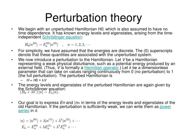
Time-dependent perturbation theory • The theory described here is essential for understanding the optical transitions from one state to another and thus spectroscopies. It gives the formula for intensities of spectral bands. • The probability of transition (intensity of a spectral band for the transition n← 0) is
Zeroth order • Before the perturbation is turned on, the system is in time-independent ground state. • Let us remember that a “time-independent” wave function does have hidden time dependence of the form:
Perturbation = light • Next, we shine light on the system. Light (or a photon) is a time-oscillating electromagnetic field. It is very weak as compared to electrostatic interactions between electrons and nuclei in atoms and molecules. It can be treated as a time-dependent perturbation: Oscillating real electrostatic field in z direction with intensity Eand angular frequency ω= 2πν.
Perturbation = light Oscillating real electrostatic field in z direction with intensity Eand angular frequency ω= 2πν.
First order • Once we turn on the time-dependent perturbation, the wave function will have time-dependent response. We consider the first-order response. We expand the first-order correction to the zeroth-order wave function by eigenfunctions of the known (initial, time-independent) system.
First order • Substituting into the time-dependent Schrödinger equation:
First order • Collecting the terms in first order in λ
First order • Using that are eigenfunctions of H(0) Cancel
First order • Multiplying from the left and integrating Cancel 1 only if n = k
First order • Simplifying 1 only if n = k Equal Energy conservation!
First order Excitation or deexcitation
First order • Removing the time-oscillating factors
Fermi’s golden rule • The probability of transition (intensity of a spectral band for the transition n← 0) is • When the dipole moment interacts with the oscillating electric field (light), the transition probability is proportional to the square of the transition dipole moment (in the direction of polarization) and square of the intensity of light.
Summary • Spectroscopic transitions can be explained by the time-dependent Schrödinger equation. One-photon transition can be understood by first-order time-dependent perturbation theory. • Energy conservation • Transition dipole moment • Intensity of light