Download
1 / 101
1.04k likes | 1.3k Views
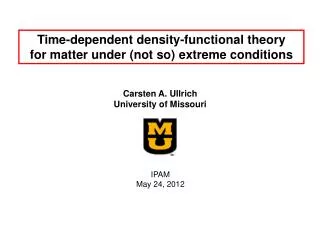
Carsten A. Ullrich University of Missouri-Columbia. Time-dependent density-functional theory. Neepa T. Maitra Hunter College & Graduate Center CUNY. APS March Meeting 2010, New Orleans. Outline. 1. A survey of time-dependent phenomena 2. Fundamental theorems in TDDFT

E N D
Carsten A. Ullrich University of Missouri-Columbia Time-dependent density-functional theory Neepa T. Maitra Hunter College & Graduate Center CUNY APS March Meeting 2010, New Orleans
Outline 1. A survey of time-dependent phenomena 2. Fundamental theorems in TDDFT 3. Time-dependent Kohn-Sham equation 4. Memory dependence 5. Linear response and excitation energies 6. Optical processes in Materials 7. Multiple and charge-transfer excitations 8. Current-TDDFT 9. Nanoscale transport 10. Strong-field processes and control C.U. N.M. C.U. N.M. N.M. C.U. N.M. C.U. C.U. N.M.
1. SurveyTime-dependent Schrödinger equation kinetic energy operator: electron interaction: The TDSE describes the time evolution of a many-body state starting from an initial state under the influence of an external time-dependent potential From now on, we’ll (mostly) use atomic units (e = m = h = 1).
1. Survey Real-time electron dynamics: first scenario Start from nonequilibrium initial state, evolve in static potential: t=0 t>0 Charge-density oscillations in metallic clusters or nanoparticles (plasmonics) New J. Chem. 30, 1121 (2006) Nature Mat. Vol. 2 No. 4 (2003)
1. SurveyReal-time electron dynamics: second scenario Start from ground state, evolve in time-dependent driving field: t=0 t>0 Nonlinear response and ionization of atoms and molecules in strong laser fields
1. Survey Coupled electron-nuclear dynamics ● Dissociation of molecules (laser or collision induced) ● Coulomb explosion of clusters ● Chemical reactions High-energy proton hitting ethene T. Burnus, M.A.L. Marques, E.K.U. Gross, Phys. Rev. A 71, 010501(R) (2005) Nuclear dynamics treated classically For a quantum treatment of nuclear dynamics within TDDFT (beyond the scope of this tutorial), see O. Butriy et al., Phys. Rev. A 76, 052514 (2007).
1. SurveyLinear response tickle the system observe how the system responds at a later time density response density-density response function perturbation
Na2 Na4 Theory Photoabsorption cross section Energy (eV) Vasiliev et al., PRB 65, 115416 (2002) 1. SurveyOptical spectroscopy ● Uses weak CW laser as Probe ● System Response has peaks at electronic excitation energies Green fluorescent protein Marques et al., PRL 90, 258101 (2003)
Outline 1. A survey of time-dependent phenomena 2. Fundamental theorems in TDDFT 3. Time-dependent Kohn-Sham equation 4. Memory dependence 5. Linear response and excitation energies 6. Optical processes in Materials 7. Multiple and charge-transfer excitations 8. Current-TDDFT 9. Nanoscale transport 10. Strong-field processes and control C.U. N.M. C.U. N.M. N.M. C.U. N.M. C.U. C.U. N.M.
Y0 2. FundamentalsRunge-Gross Theorem kinetic external potential For any system with Hamiltonian of form H = T + W + Vext , e-e interaction • Runge & Gross (1984) proved the 1-1 mapping for fixed T and W: • n(r t)vext(r t) • For a given initial-statey0, the time-evolving one-body density n(r t) tells you everything about the time-evolving interacting electronic system, exactly. This follows from : Y0, n(r,t) unique vext(r,t) H(t) Y(t) all observables
vext(t), Y(t) Yo vext’(t), Y’(t) same 2. FundamentalsProof of theRunge-Gross Theorem (1/4) Consider two systems of N interacting electrons, both starting in the same Y0 , but evolving under different potentials vext(r,t) and vext’(r,t) respectively: Assume time-analytic potentials: RG prove that the resulting densities n(r,t) and n’(r,t) eventually must differ, i.e.
;t ) 2. FundamentalsProof of theRunge-Gross Theorem (2/4) The first part of the proof shows that the current-densities must differ. Consider Heisenberg e.o.m for the current-density in each system, the part of H that differs in the two systems At the initial time: initial density if initially the 2 potentials differ, thenj and j’ differ infinitesimally later ☺
1-1 • provesj(r,t)vext(r,t) Yo 2. FundamentalsProof of theRunge-Gross Theorem (3/4) If vext(r,0) = v’ext(r,0), then look at later times by repeatedly using Heisenberg e.o.m : … * Asvext(r,t) – v’ext(r,t) = c(t), and assuming potentials are time-analytic at t=0, there must be somekfor which RHS = 0 • 1st part of RG ☺ The second part of RG proves 1-1 between densities and potentials: Take divergence of both sides of * and use the eqn of continuity, …
same 2. FundamentalsProof of theRunge-Gross Theorem (4/4) … ≡ u(r) is nonzero for some k, but must taking the div here be nonzero? Yes! By reductio ad absurdum: assume assume fall-off of n0 rapid enough that surface-integral 0 Then integrand0, so if integral 0, then contradiction i.e. • 1-1 mapping between time-dependent densities and potentials, for a given initial state
2. FundamentalsThe TDKS system • n v for given Y0, implies any observable is a functional of n and Y0 • -- So map interacting system to a non-interacting (Kohn-Sham) one, that reproduces the same n(r,t). • All properties of the true system can be extracted from TDKS “bigger-faster-cheaper” calculations of spectra and dynamics • KS “electrons” evolve in the 1-body KS potential: • functional of the history of the density • and the initial states • -- memory-dependence (see more shortly!) • If begin in ground-state, then no initial-state dependence, since by HK, • Y0 = Y0[n(0)] (eg. in linear response). Then
2. FundamentalsClarifications and Extensions • But how do we know a non-interacting system exists that reproduces a given interacting evolution n(r,t) ? • van Leeuwen (PRL, 1999) for time-analytic potentials and densities • (& under mild restrictions of the choice of the KS initial state F0) • The KS potential is not the density-functional derivative of any action ! • If it were, causality would be violated: • Vxc[n,Y0,F0](r,t) must be causal – i.e. cannot depend on n(r t’>t) • But if then • But RHS must be symmetric in (t,t’) symmetry-causality paradox. • van Leeuwen (PRL 1998): an action, and variational principle, may be defined, using Keldysh contours in complex-time. • Vignale (PRA 2008): usual real-time action is just fine IF include boundary terms
2. FundamentalsClarifications and Extensions • Restriction to time-analytic potentials means RG is technically not valid for many potentials, eg adiabatic turn-on, although RG is assumed in practise. • van Leeuwen (Int. J. Mod. Phys. B. 2001) extended the RG proof in the linear response regime to the wider class of Laplace-transformable potentials. • The first step of the RG proof showed a 1-1 mapping between currents and potentials TD current-density FT • In principle, must use TDCDFT (not TDDFT) for • -- response of periodic systems (solids) in uniform E-fields (see later…) • -- in presence of external magnetic fields(Ghosh & Dhara, PRA 1988) • In practice, approximate functionals of current are simpler where spatial non-local dependence is important • (Vignale & Kohn, 1996; Vignale, Ullrich & Conti 1997)… Stay tuned!
Outline 1. A survey of time-dependent phenomena 2. Fundamental theorems in TDDFT 3. Time-dependent Kohn-Sham equation 4. Memory dependence 5. Linear response and excitation energies 6. Optical processes in Materials 7. Multiple and charge-transfer excitations 8. Current-TDDFT 9. Nanoscale transport 10. Strong-field processes and control C.U. N.M. C.U. N.M. N.M. C.U. N.M. C.U. C.U. N.M.
3. TDKSTime-dependent Kohn-Sham scheme (1) Consider anN-electron system, starting from a stationary state. Solve a set of static KS equations to get a set of N ground-state orbitals: The N static KS orbitals are taken as initial orbitals and will be propagated in time: Time-dependent density:
3. TDKSTime-dependent Kohn-Sham scheme (2) Only the N initially occupied orbitals are propagated. How can this be sufficient to describe all possible excitation processes?? Here’s a simple argument: Expand TDKS orbitals in complete basis of static KS orbitals, finite for A time-dependent potential causes the TDKS orbitals to acquire admixtures of initially unoccupied orbitals.
depends on density at time t (instantaneous, no memory) is a functional of The time-dependent xc potential has a memory! 3. TDKSAdiabatic approximation Adiabatic approximation: (Take xc functional from static DFT and evaluate with time-dependent density) ALDA:
time 3. TDKSTime-dependent selfconsistency (1) start with selfconsistent KS ground state propagate until here I. Propagate II. With the density calculate the new KS potential for all III. Selfconsistency is reached if
3. TDKSNumerical time Propagation Propagate a time step Crank-Nicholson algorithm: Problem: must be evaluated at the mid point But we know the density only for times
3. TDKSTime-dependent selfconsistency (2) Predictor Step: nth Corrector Step: Selfconsistency is reached if remains unchanged for upon addition of another corrector step in the time propagation.
1 2 3 3. TDKSSummary of TDKS scheme: 3 Steps Prepare the initial state, usually the ground state, by a static DFT calculation. This gives the initial orbitals: Solve TDKS equations selfconsistently, using an approximate time-dependent xc potential which matches the static one used in step 1. This gives the TDKS orbitals: Calculate the relevant observable(s) as a functional of
initial-state density hard walls periodic boundaries (travelling waves) exact LDA z x (standing waves) Charge-density oscillations Δ L 3. TDKSExample: two electrons on a 2D quantum strip ● Initial state: constant electric field, which is suddenly switched off ● After switch-off, free propagation of the charge-density oscillations C.A. Ullrich, J. Chem. Phys. 125, 234108 (2006)
3. TDKSConstruction of the exact xc potential Step 1: solve full 2-electron Schrödinger equation Step 2: calculate the exact time-dependent density Step 3: find that TDKS system which reproduces the density
density adiabatic Vxc exact Vxc 3. TDKS2D quantum strip: charge-density oscillations ● The TD xc potential can be constructed from a TD density ● Adiabatic approximations get most of the qualitative behavior right, but there are clear indications of nonadiabatic (memory) effects ● Nonadiabatic xc effects can become important (see later)
Outline 1. A survey of time-dependent phenomena 2. Fundamental theorems in TDDFT 3. Time-dependent Kohn-Sham equation 4. Memory dependence 5. Linear response and excitation energies 6. Optical processes in Materials 7. Multiple and charge-transfer excitations 8. Current-TDDFT 9. Nanoscale transport 10. Strong-field processes and control C.U. N.M. C.U. N.M. N.M. C.U. N.M. C.U. C.U. N.M.
4. Memory Memory dependence functional dependence on history, n(r t’<t), and on initial states Maitra, Burke, Woodward (PRL 2002): Exact condition relating initial-state dependence and history-dependence. Almost all calculations ignore memory, and use an “adiabatic approximation” : Just take xc functional from static DFT and evaluate on instantaneous density vxc But what about the exact functional?
4. Memory Example of history dependence Eg. Time-dependent Hooke’s atom –exactly solvable 2 electrons in parabolic well, time-varying force constant k(t) =0.25 – 0.1*cos(0.75 t) parametrizesdensity Any adiabatic (or even semi-local-in-time) approximation would incorrectly predict the same vc at both times. Hessler, Maitra, Burke, (J. Chem. Phys, 2002); see also other examples in the Literature handout • Development of History-Dependent Functionals: Dobson, Bunner & Gross (1997), Vignale, Ullrich, & Conti (1997), Kurzweil & Baer (2004), Tokatly (2005,2007)
Y0 RG: n(r t) vext(r t) 1-1 n (r t) ~ ~ ? Evolve Y0 in v (t) same n ? 4. Memory Initial-state dependence But is there ISD?That is, if we start in different Y0’s, can we get the same n(r t), for all t, by evolving in different potentials? i.e. Evolve Y0 in v(t) The answer is: No! for one electron, but, Yes! for 2 or more electrons t If no, then ISD redundant, i.e. the functional dependence on the density is enough.
4. Memory Example of initial-state dependence A non-interacting example: Periodically driven HO Re and Im parts of 1st and 2nd Floquet orbitals If we start in different Y0’s, can we get the same n(r t) by evolving in different potentials? Yes! Doubly-occupied Floquet orbital with same n • Say this is the density of an interacting system. Both top and middle are possible KS systems. • vxc different for each. Cannot be captured by any adiabatic approximation ( Consequence for Floquet DFT: No 1-1 mapping between densities and time-periodic potentials. ) Maitra & Burke, (PRA 2001)(2001, E); Chem. Phys. Lett. (2002).
4. Memory Time-dependent optimized effective potential where exact exchange: C.A.Ullrich, U.J. Gossmann, E.K.U. Gross, PRL 74, 872 (1995) H.O. Wijewardane and C.A. Ullrich, PRL 100, 056404 (2008)
Outline 1. A survey of time-dependent phenomena 2. Fundamental theorems in TDDFT 3. Time-dependent Kohn-Sham equation 4. Memory dependence 5. Linear response and excitation energies 6. Optical processes in Materials 7. Multiple and charge-transfer excitations 8. Current-TDDFT 9. Nanoscale transport 10. Strong-field processes and control C.U. N.M. C.U. N.M. N.M. C.U. N.M. C.U. C.U. N.M.
Poles at true excitations Poles at KS excitations adiabatic approx: no w-dep 5. Linear ResponseTDDFT in linear response Need (1) ground-state vS,0[n0](r), and its bare excitations (2) XC kernel Yields exact spectra in principle; in practice, approxs needed in (1) and (2). Petersilka, Gossmann, Gross, (PRL, 1996)
5. Linear ResponseMatrix equations (a.k.a. Casida’s equations) Quantum chemistry codes cast eqns into a matrix of coupled KS single excitations (Casida 1996) : Diagonalize q = (i a) Excitation energies and oscillator strengths Useful tools for analysis: “single-pole” and “small-matrix” approximations (SPA,SMA) Zoom in on a single KS excitation, q = i a Well-separated single excitations: SMA When shift from bare KS small: SPA
LDA + ALDA lowest excitations SPA SMA Exp. full matrix Vasiliev, Ogut, Chelikowsky, PRL 82, 1919 (1999) 5. Linear ResponseHow it works: atomic excitation energies TDDFT linear response from exact helium KS ground state: Compare different functional approxs (ALDA, EXX), and also with SPA. All quite similar for He. From Burke & Gross, (1998); Burke, Petersilka & Gross (2000)
5. Linear ResponseAtomic excitations: Rydberg states Generally, KS excitations themselves are good zero-order approximations to the exact energies – except when they are missing! LDA/GGA KS potentials asymptotically decay exponentially (ground-state lectures) No -1/r tail no Rydberg excitations. Either paste a tail on (eg LB94, or some kind of hybrid…) OR, use a clever trick to obtain their energies: Quantum defect theory: determined by short-range part of v A. Wasserman & K. Burke, Phys. Rev. Lett. (2005);
5. Linear ResponseA comparison of functionals Study of various functionals over a set of ~ 500 organic compounds, 700 excited singlet states From: D. Jacquemin, V. Wathelet, E. A. Perpete, C. Adamo, J. Chem. Theory Comput. (2009).
5. Linear response General trends • Energies typically to within about “0.4 eV” • Bonds to within about 1% • Dipoles good to about 5% • Vibrational frequencies good to 5% • Cost scales as N3, vs N5 for wavefunction methods of comparable accuracy (eg CCSD, CASSCF) • Available now in many electronic structure codes • Unprecedented balance between accuracy and efficiency TDDFT Sales Tag
5. Linear response Examples Can study big molecules with TDDFT ! carotenoid-diaryl-porphyrin-C60 -- Can study candidates for solar cells, eg. (632 valence electrons! ) Photo-excitation of a light-harvesting supra-molecular triad: a TDDFT study, N. Spallanzani, C. A. Rozzi, D. Varsano, T. Baruah, M. R. Pederson, F. Manghi, and A. Rubio, J. Phys. Chem. (2009)
5. Linear response Examples Circular dichroism spectra of chiral fullerenes: D2C84 F. Furche and R. Ahlrichs, JACS 124, 3804 (2002).
Outline 1. A survey of time-dependent phenomena 2. Fundamental theorems in TDDFT 3. Time-dependent Kohn-Sham equation 4. Memory dependence 5. Linear response and excitation energies 6. Optical processes in Materials 7. Multiple and charge-transfer excitations 8. Current-TDDFT 9. Nanoscale transport 10. Strong-field processes and control C.U. N.M. C.U. N.M. N.M. C.U. N.M. C.U. C.U. N.M.
finite extended x x x x x 6. TDDFT in solids Excitations in finite and extended systems The full many-body response function has poles at the exact excitation energies ► Discrete single-particle excitations merge into a continuum (branch cut in frequency plane) ► New types of collective excitations appear off the real axis (finite lifetimes)
6. TDDFT in solids Metals vs. insulators plasmon Excitation spectrum of simple metals: ● single particle-hole continuum (incoherent) ● collective plasmon mode Optical excitations of insulators: ● interband transitions ● excitons (bound electron-hole pairs)
6. TDDFT in solids Excitations in bulk metals Plasmon dispersion of Al Quong and Eguiluz, PRL 70, 3955 (1993) ►RPA (i.e., Hartree) gives already reasonably good agreement ►ALDA agrees very well with exp. In general, (optical) excitation processes in (simple) metals are very well described by TDDFT within ALDA. Time-dependent Hartree already gives the dominant contribution, and fxc typically gives some (minor) corrections. This is also the case for 2DEGs in doped semiconductor heterostructures (quantum wells, quantum dots).
6. TDDFT in solids Elementary view of excitons Excitons are bound electron-hole pairs created in optical excitations of insulators. Mott-Wannier exciton: weakly bound, delocalized over many lattice constants Frenkel exciton: tightly bound, localized on a single (or a few) atoms
GaAs Cu2O R.G. Ulbrich, Adv. Solid State Phys. 25, 299 (1985) R.J. Uihlein, D. Frohlich, and R. Kenklies, PRB 23, 2731 (1981) 6. TDDFT in solids Wannier equation and excitonic Rydberg series ● is exciton wave function ● derived from TDHF linearized Semiconductor Bloch equation ● includes dielectric screening