Download
1 / 45
450 likes | 531 Views
Enhancing locality in ray tracing algorithms. 612 presentations by Vidhyashankar Venkataraman Biswanath Panda. Introduction. Two-lecture series We will be discussing two methods to preserve locality By processing data groups that are likely to be accessed at the same time

E N D
Enhancing locality in ray tracing algorithms 612 presentations by Vidhyashankar Venkataraman Biswanath Panda
Introduction • Two-lecture series • We will be discussing two methods to preserve locality • By processing data groups that are likely to be accessed at the same time • Today : A locality-aware algorithm in ray tracing
What is Computer Graphics (CG)? • Generating images • Lots of cool ones in this talk! • Deals with • Geometric modeling : The math and physics • Rendering : Model to images • Animation : Time dependent behavior of objects • Applications in games, real world simulations, CAD
Rendering an image • Produce scene image on the image plane • Three parts: • Geometry Modeling • Illumination of objects • Surface complexity : Texture
1) Modeling geometry • Regular objects easy to represent • Eg. Sphere (R,x,y,z) • Complicated objects through a ‘mesh’ of polygons • Millions of primitives for a single scene
2) Illumination modeling : Shading • Lighting of objects (shading) • Light energy absorbed, reflected or transmitted • Degree varies with nature of each object • Expressed for R,G,B • Various aspects to think of • Diffuse and specular lighting • Refraction • Shadows • Mathematical models available
3) Surface complexity - Texture • To represent surface roughness • The ‘jaggedness’ • Texture map : Simple 2-D to 3-D surface • Can add geometric detail • Difficult with polygons • Also used to represent complicated surfaces • Eg: Marbles • Reflection of a scene on a complex polished surface • Storage Complexity? • 100s of KB to 100s of MB!
Rendering an image • Process of converting 3-D scene to actual image • Projection of the 3-D objects onto an image plane • Global illumination : more realistic • Various methods available • Ray-tracing • Scan-line conversion
Ray tracing • Introduced in 1980 by Turner Whitted • First global illumination algorithm • Insight : To find the color of each pixel : Backtracing • Trace rays from eye (pixel) into scene • Rays intersect with objects and get reflected or transmitted • Shadows, reflection, refractions
Algorithm in pictures Single intersection with object No intersection Intersected object could be directly illuminated
Algorithm in Pictures Shadow region Reflection
Algorithm in pictures Refraction : Transmission of rays Multiple reflections
In short… • Shoot ray from eye through pixel into the scene • Obtain intersection point if any • Spawn off new rays in the incident directions wrt reflection, refraction, direct lighting or through shadows • Color of pixel is the sum of light energies of all of them (called the radiance) • The secondary rays will also spawn off new rays : Recursively performed
The algorithm in text • For each pixel (x,y) in image, generate corresponding ray in 3D • Image(x,y) := TraceRay(ray) • TraceRay(ray) 1) Compute nearest surface-ray intersection 2) If none found return background color 3) Compute direct illumination from eachlight source 4) Compute illumination arriving from reflected direction 5) Compute illumination arriving from refracted direction 6) Combine all illuminations 7) Return resulting color • Step 3 involves testing visibility of source by shooting shadow ray towards it • Steps 4 and 5 involve recursive calls to TraceRay using corresponding rays
The ray tree Recursive calls represented as a tree
RT : Backward Tracing First ray-traced image
Surface-ray intersection • Most important part • Closest intersection • Surface primitives : polygons, spheres, cubes • Too expensive to test for each surface primitive in scene • Moving GB of geometry in and out of memory! • Optimizations : • Curb depth of tree • Faster and fewer intersection calculations • Bounding volume of each object by some regular shape (sphere / cube) • Spatial Subdivision (discussed in next slide)
Optimizations – ‘Voxel’ subdivision Adaptive subdivision (Octree) Uniform subdivision Voxel is a 3-D sub-region of a scene
Issues in rendering • Pros and cons of RT • Pros : • Almost accurately lit if tree is sufficiently deep • Simple algorithm • Cons : • For faster rendering, standard traversals may not be coherent, hence can lead to a large number of page faults • Other rendering algorithm • Scan-line based : Can render complex scenes • Inaccurate illumination : Very unrealistic • Much faster than RT • Advent of GPUs • Processors exclusively for CG : Faster rendering • Parallelism and pipelining • Aggressive prefetching from memory
Examples of Scan Conversion Poor lighting; More use of texture maps A more memory-coherent RT algorithm could improve things
Enough of intro… • 612 in CG! • Enhance locality in RT to avoid memory issues • Take this! An image having 10 million primitives with 400 MB geometry • Involved 2 GB of I/O! Took 5 hours of rendering with RT! • First paper in two lecture series : Pharr et al. (SIGGRAPH ‘97) • Lazy creation of texture and geometry to manage scene complexity : Caching in main memory • Increase locality of reference by dynamically reordering rendering computation
Essential Ideas • Statically reorder geometry into voxels of triangles • Remember voxels? Uniform 3-D cubes enclosing some geometry • Maintain geometry cache • Texture data pre filtered and cached • Application-level caching • Process one bunch of rays after another (from queue) • Rays partitioned into coherent groups • Calculate illumination wherever rays intersect, possibly spawn new ones and queue them • Terminate if all rays finished
Scheduling of rays - Reordering • Goal : To process rays in particular order so as to • Minimize cache misses (here, page faults) • Advance computation towards completion • Each queued ray to be independent of result or state of other rays • Take advantage of the illumination computation
Decompose Computation • Illumination computation at point x in direction w1 is of the form: • Lo(x, wr) = Le(x, wr) + Σ W(x, wi, wr, Θi) Li(x, wi) Where • Lo = Outgoing radiance • Le = Emitted radiance • Li = Incoming radiance through direction wi hitting at x • Θi = Angle between wi and surface normal at x • W is a factor that depends on the material of x and whether there is reflection or refraction • We can successively multiply the W’s as we go down the tree!
Decompose Computation • Each ray associated with weight and source pixel location • Spawned ray’s weight multiplied by weight of parent ray • If ray hits light source weight multiplied and result added to source pixel W1 W3 W3.W4 W1.W2 W3.W5
Ray Grouping • Closely spaced rays likely to intersect closely spaced geometry primitives • Scene uniformly divided into another grid of voxels : scheduling grid • Each voxel has following state • Queue of rays passing through it • The geometry voxels overlapping it • Voxel with highest ratio of benefit to cost chosen by scheduler • For each ray in queue, test for intersection in voxel • If yes, calculate illumination and spawn new rays • Else, queue it up in next voxel
Issues : Size of scheduling voxel • Scheduling voxel : small enough for overlapping geometry voxel to fit into memory • Non-uniform geometry : Can use adaptive subdivision (octree) • Avoid geometry cache misses (page faults) • Schedule voxels that have all geometry in cache • Defer processing rays that don’t have geometry in cache • Lots of rays then : Have ray cache as well
Issues : Voxel Scheduling • Choose voxel with highest ratio of benefit to cost • Cost : • How much overlapping geometry not in cache • Difficult to estimate apriori if lazy access • Reduce cost a lot (by 90%) if all geometry in cache • Benefit : • How much towards completion • Number of rays , their weights? • The weighted sum?
Scene cache • Geometry represented as mesh of triangles • Even spheres, cubes..! • For ease of sub dividing into voxels • Only one kind of intersection test • Storage of geometry: • Δgle meshes stored as voxels in disk • Tessellated patches also as triangles • Procedurally generated geometry • Texture-based data stored as extra geometry
Scene cache • Size of geometry cache in main memory • Make volume of voxel roughly equal to size of block • Few thousands of Δgles per voxel • Divided into sub-voxel for ray intersection acceleration • Remember voxels may not occupy same space • To avoid fragmentation special allocation routines written
Texture Cache • Similar to one proposed earlier by Peachey • Texture data pre-filtered into set of multi resolution images • Choose image depending on resolution of texture • Called mip-maps • Shading calculation of a pixel makes a small number of accesses to some local part of texture
Results • Experiments performed on 190 MHz MIPS R10000 processor with 1 GB of memory • I/O buffering disabled to increase memory constraints • Scenes occupy between 431 MB and 1.9 GB
Rendered scenes – Tree by lake • Maximum of 3.3 million triangles for the tree • Terrain and lake used displacement mapping : more number of triangles • Total of 9.6 million primitives : 440 MB needed • 677 X 288 resolution
Rendered scenes – Office building • Very complex scene with dense occlusions • Office Building has two floors with four offices • 46.4 million primitives with 1.9 GB of memory • Lit by sunlight and some lights in ceiling • 672 X 384 resolution
Rendered Scenes - Cathedral • Base 11K Triangles; With displacement map : 5.1 million primitives! A total of 431 MB • 576 X 864 resolution • 1495 texture maps of 116 MB! • Simple lighting source
Caching but no reordering • Unlimited cache size but with lazy loading • Both memory and running time costs decrease • 22% memory use reduction in Cathedral case (not accessed) • Only 18% of total scene accessed in indoor case • Obvious result!
Caching but no reordering • Performance of geometry caching when DFS Ray tracing is used • Limited cache size • Performance decrease not very significant
Scheduling & Reordering 80% of scene memory • Rendering Lake scene • Cache size of 10% of maximum gives orders of magnitude performance gain • Ray cache of 100K rays (6% of total number of rays)
Scheduling and Reordering Accessed 15-20 times • Lake scene rendering • Without reordering and 325MB of geometry cache, 2.1 GB of I/O! • With reordering and 50 MB cache, 938 MB in total Average access = 8 times
Conclusions • Enhance locality in RT through caching and reordering • Gives orders of magnitude performance gain • Algorithm performs well! • Ideas not very seminal.. But the work is! • Future work : Experiments could be redone on the IBM Cell Processor to confirm the bottlenecks • Designed for PlayStation3 • 4.6 GHz specialized graphics processors… • Next lecture : A static method to perform data grouping