Download
1 / 40
430 likes | 625 Views
ECTE461 – Telecommunications Queuing Theory. Mathematical analysis of telecommunications switch performance. Assessment. Queuing Systems. Queue at supermarket – FIFO (first in first out) with single server Queue at NAB – FIFO with multiple servers (tellers)

E N D
ECTE461 – Telecommunications Queuing Theory Mathematical analysis of telecommunications switch performance
Queuing Systems • Queue at supermarket – FIFO (first in first out) with single server • Queue at NAB – FIFO with multiple servers (tellers) • Inventories at warehouse or grocer – FIFO • Packets arriving at switch – FIFO • Phone callers trying to get a line – FIFO with multiple servers
FIFO Queues Single server Multiple servers
Nature of Queue • Usually FIFO. Newcomers get on the end of the queue. When they reach the front of the line, they are served • Queue can be empty, but in general it has some non-negative integer number of members • There may be a maximum number of spaces
New Arrivals • We never know just when a new member will arrive to be added to a queue • We assume that new arrivals can be described in terms of probability • For example, the probability of a new member arriving in the next second is 0.4
Probability • Something which we are certain will not happen has a probability of 0 • Something which will happen for certain has a probability of 1.0 • A probability of 0.4 means that after a long (theoretically infinite) run of tests, the event will have happened in 40% of cases
Probability • If there are n possible outcomes, and the probability of the ith outcome is pi, then • It is possible for n to go to ∞
Probability • If each possible outcome represents a number, ki, then the expected value, on the average is • Again, n may go to ∞
Combined Events • If the probabilities of two independent events are p1 and p2, then the probability of both of them occurring is p1p2 • Consider a total of N pairs of these events. In p1N cases, event 1 has occurred. In a fraction, p2 of these, event 2 has also occurred; ie p1p2N
Conditional Probability • Event 1 = e1, event 2 = e2 • The probability of e1 and e2 occurring, given that we know that e1 has already occurred, is simply p2 • P(e1 and e2) = p1p2 • P(e1 and e2|e1) = p2 = p1p2/p1 = P(e1 and e2)/P(e1)
Arrival of Packets • e1 = packet arrives after period, a • e2 = packet arrives after a + b • e3 = packet arrives after b a b t=0 time, t
Arrival of Packets • If the packet does not arrive until a + b, then it necessarily does not arrive before a. • That is if e2 occurs, then e1 has necessarily occurred, since a + b > a. • So P(e1 and e2) = P(e2) and • P(e1 and e2|e1) = P(e2|e1)
Arrival of Packets • If we know that no packet has arrived at t = a, then the probability that a packet will not arrive until t = a + b is simply p3, the probability that a packet will not arrive before a time of b has elapsed • Ie, P(e2|e1) = p3
Arrival of Packets • The conditional probability formula gives • P(e1 and e2|e1) = P(e1 and e2)/P(e1) • Ie, P(e3) = P(e2)/P(e1) • Ie, p2 = p1p3 • We can re-write this as follows
Exponential Distribution • P(packet does not arrive before a + b) = P(packet does not arrive before a) x P(packet does not arrive before b) • We could write this as • P(a + b) = P(a) P(b) • Then put a = t and b = dt, to give • P(t + dt) = P(t) P(dt)
Exponential Distribution • Now probability that packet arrives in time dt is ldt • So P(dt) = 1 – ldt • And P(t + dt) = P(t) + dt • So we have • P(t) + dt = P(t)(1 – ldt)
Exponential Distribution • This gives us • = -l P(t) • which leads to • P(t) = e-lt + const • Since P(0) = 1, const = 0
Exponential Distribution • P(t) = e-lt • That is, if the probability of a packet arriving in any small time interval, dt is ldt, then the probability of the next packet arriving after time, t, is e-lt • This is called the exponential distribution
Exponential Distribution • This distribution is “memoryless”: that is, it is not changed by what has happened before. At every point in time, the probability of the next packet arriving after t is e-lt • Many situations can be described by this process, to a reasonable degree of accuracy
Exponential Distribution • Real time traffic is often close to exponential distribution • This is not always the case. If the traffic is “bursty”, then earlier events change the probability • This is frequently the case with data traffic
Exponential Distribution • If we have a time, t = a + b, then • P(t) = e-lt = e-l(a+b) = e-lae-lb = P(a)P(b) (as we assumed to begin)
Poisson and Markov • The process which produces the exponential distribution is called a “Poisson” process • A Markov “chain” is a chain of events described by an exponential probability distribution • Both of these terms will be used
Poisson Process • How many packets do we expect to arrive in an interval, T? • What is the average arrival rate of packets in a Poisson process? • To answer these questions, and others, we need to find the probability of k packets arriving in T
Poisson Process • We divide T into m very short intervals, Dt • The probability of one packet arriving in one of these intervals is lDt • The probability of no packets arriving is 1 – lDt • We ignore the possibility of more than one packet arriving (O(Dt2))
Poisson Process • In order to get k packets arriving, we need one packet to arrive in each of k of the m short intervals • For any particular combination of these intervals, the probability is • (lDt)k x (1 – lDt)m-k
Poisson Process • The number of different combinations of k intervals out of a total of m intervals is • This is the coefficient for the binomial expansion
Poisson Process • So the probability is • As m becomes very large, and Dt k becomes very small compared to m • So m!/(m-k)! ≈ mk
Poisson Process • Since mDt = T, the probability can be re-written
Poisson Process • So we can write the probability
Poisson Process • Remember, this was the probability that k packets would arrive in a period, T • It is called the Poisson distribution
Example • To three decimal places, what are the probabilities of 0, 1, 2, …10 packets arriving in the period T = 1/l? • Here we have • The first 11 values are 0.368, 0.368, 0.184, 0.061, 0.015, 0.003, 0.000,…
Exponential and Poisson • If we put k = 0, we have the probability that no packets arrive in the interval, T • We see that the exponential distribution is a special case of the Poisson • P(0) = e-lT
Poisson Process • We can now calculate the average, or expected number of packets arriving during T • We use the formula for the average of a set of possible outcomes (from before)
Poisson Process • The term for k = 0 is zero. We then replace k-1 with j to get
Poisson Process • That is, the expected, or average number of packets arriving in time, T is just lT • This means that the average rate of arrivals is l packets per second
And Finally • We can use a similar method to show that • And the variance is