Download
1 / 68
690 likes | 933 Views
Modeling using queuing theory. if N.R=M then input capacity = capacity of multiplexed link => TDM if N.R>M but .N.R<M then this may be modeled by a queuing system to analyze its performance. Queuing system for single server. Inputs/Outputs of Queuing Theory. Given: arrival rate

E N D
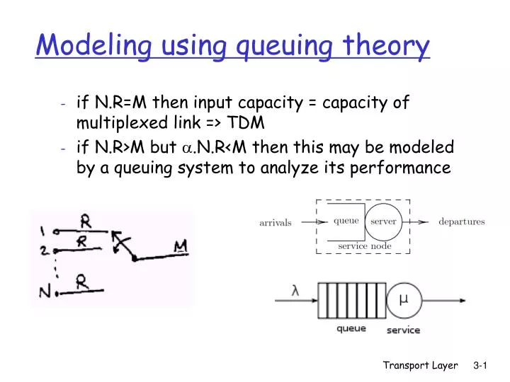
Modeling using queuing theory • if N.R=M then input capacity = capacity of multiplexed link => TDM • if N.R>M but .N.R<M then this may be modeled by a queuing system to analyze its performance Transport Layer
Queuing system for single server Transport Layer
Inputs/Outputs of Queuing Theory • Given: • arrival rate • service time • queuing discipline • Output: • wait time, and queuing delay • waiting items, and queued items Transport Layer
As increases, so do buffer requirements and delay • The buffer size ‘q’ only depends on Transport Layer
Queuing Example • If N=10, R=100, =0.4, M=500 • Or N=100, M=5000 • =.N.R/M=0.8, q=2.4 • a smaller amount of buffer space per source is needed to handle larger number of sources • variance of q increases with • For a finite buffer: probability of loss increases with utilization >0.8 undesirable Transport Layer
Chapter 3Transport Layer Computer Networking: A Top Down Approach 4th edition. Jim Kurose, Keith RossAddison-Wesley, July 2007. Computer Networking: A Top Down Approach, 5th edition. Jim Kurose, Keith RossAddison-Wesley, April 2009. Transport Layer
reliable, in-order delivery to app: TCP congestion control flow control connection setup unreliable, unordered delivery to app: UDP no-frills extension of “best-effort” IP services not available: delay guarantees bandwidth guarantees application transport network data link physical application transport network data link physical network data link physical network data link physical network data link physical network data link physical network data link physical network data link physical logical end-end transport Internet transport-layer protocols Transport Layer
Create sockets with port numbers: DatagramSocket mySocket1 = new DatagramSocket(12534); DatagramSocket mySocket2 = new DatagramSocket(12535); UDP socket identified by two-tuple: (dest IP address, dest port number) When host receives UDP segment: checks destination port number in segment directs UDP segment to socket with that port number IP datagrams with different source IP addresses and/or source port numbers directed to same socket Connectionless demultiplexing Transport Layer
P3 P2 P1 P1 SP: 9157 client IP: A DP: 6428 Client IP:B server IP: C SP: 5775 SP: 6428 SP: 6428 DP: 6428 DP: 9157 DP: 5775 Connectionless demux (cont) DatagramSocket serverSocket = new DatagramSocket(6428); SP provides “return address” Transport Layer
TCP socket identified by 4-tuple: source IP address source port number dest IP address dest port number recv host uses all four values to direct segment to appropriate socket Server host may support many simultaneous TCP sockets: each socket identified by its own 4-tuple Web servers have different sockets for each connecting client non-persistent HTTP will have different socket for each request Connection-oriented demux Transport Layer
SP: 9157 SP: 5775 P1 P1 P2 P4 P3 P6 P5 client IP: A DP: 80 DP: 80 Connection-oriented demux (cont) S-IP: B D-IP:C SP: 9157 DP: 80 Client IP:B server IP: C S-IP: A S-IP: B D-IP:C D-IP:C Transport Layer
important in app., transport, link layers top-10 list of important networking topics! characteristics of unreliable channel will determine complexity of reliable data transfer protocol (rdt) Principles of Reliable data transfer Transport Layer
rdt_send():called from above, (e.g., by app.). Passed data to deliver to receiver upper layer deliver_data():called by rdt to deliver data to upper udt_send():called by rdt, to transfer packet over unreliable channel to receiver rdt_rcv():called when packet arrives on rcv-side of channel Reliable data transfer: getting started send side receive side Transport Layer
Hop-by-hop flow control • Approaches/techniques for hop-by-hop flow control • Stop-and-wait • sliding window • Go back N • Selective reject Transport Layer
underlying channel perfectly reliable no bit errors, no loss of packets stop and wait Stop-and-wait: reliable transfer over a reliable channel Sender sends one packet, then waits for receiver response Transport Layer
underlying channel may flip bits in packet checksum to detect bit errors the question: how to recover from errors: acknowledgements (ACKs): receiver explicitly tells sender that pkt received OK negative acknowledgements (NAKs): receiver explicitly tells sender that pkt had errors sender retransmits pkt on receipt of NAK new mechanisms for: error detection receiver feedback: control msgs (ACK,NAK) rcvr->sender channel with bit errors Transport Layer
Stop-and-wait with lost packet/frame Transport Layer
Stop and wait performance • utilization – fraction of time sender busy sending • ideal case (error free) • u=Tframe/(Tframe+2Tprop)=1/(1+2a), a=Tprop/Tframe Transport Layer
Pipelining: sender allows multiple, “in-flight”, yet-to-be-acknowledged pkts range of sequence numbers must be increased buffering at sender and/or receiver Two generic forms of pipelined protocols: go-Back-N, selective repeat Pipelined (sliding window) protocols Transport Layer
Pipelining: increased utilization sender receiver first packet bit transmitted, t = 0 last bit transmitted, t = L / R first packet bit arrives RTT last packet bit arrives, send ACK last bit of 2nd packet arrives, send ACK last bit of 3rd packet arrives, send ACK ACK arrives, send next packet, t = RTT + L / R Increase utilization by a factor of 3! Transport Layer
Sender: k-bit seq # in pkt header “window” of up to N, consecutive unack’ed pkts allowed Go-Back-N • ACK(n): ACKs all pkts up to, including seq # n - “cumulative ACK” • may receive duplicate ACKs (more later…) • timer for each in-flight pkt • timeout(n): retransmit pkt n and all higher seq # pkts in window Transport Layer
GBN inaction Transport Layer
receiver individually acknowledges all correctly received pkts buffers pkts, as needed, for eventual in-order delivery to upper layer sender only resends pkts for which ACK not received sender timer for each unACKed pkt sender window N consecutive seq #’s limits seq #s of sent, unACKed pkts Selective Repeat Transport Layer
Selective repeat: sender, receiver windows Transport Layer
Selective repeat in action Transport Layer
performance: • selective repeat: • error-free case: • if the window is w such that the pipe is fullU=100% • otherwise U=w*Ustop-and-wait=w/(1+2a) • in case of error: • if w fills the pipe U=1-p • otherwise U=w*Ustop-and-wait=w(1-p)/(1+2a) Transport Layer
full duplex data: bi-directional data flow in same connection MSS: maximum segment size connection-oriented: handshaking (exchange of control msgs) init’s sender, receiver state before data exchange flow controlled: sender will not overwhelm receiver point-to-point: one sender, one receiver reliable, in-order byte stream: no “message boundaries” pipelined: TCP congestion and flow control set window size send & receive buffers TCP: OverviewRFCs: 793, 1122, 1323, 2018, 2581 Transport Layer
32 bits source port # dest port # sequence number acknowledgement number head len not used Receive window U A P R S F checksum Urg data pnter Options (variable length) application data (variable length) TCP segment structure URG: urgent data (generally not used) counting by bytes of data (not segments!) ACK: ACK # valid PSH: push data now (generally not used) # bytes rcvr willing to accept RST, SYN, FIN: connection estab (setup, teardown commands) Internet checksum (as in UDP) Transport Layer
Reliability in TCP • Components of reliability • 1. Sequence numbers • 2. Retransmissions • 3. Timeout Mechanism(s): function of the round trip time (RTT) between the two hosts (is it static?) Transport Layer
TCP Round Trip Time and Timeout EstimatedRTT(k) = (1- )*EstimatedRTT(k-1) + *SampleRTT(k) =(1- )*((1- )*EstimatedRTT(k-2)+ *SampleRTT(k-1))+ *SampleRTT(k) =(1- )k *SampleRTT(0)+ (1- )k-1 *SampleRTT)(1)+…+ *SampleRTT(k) • Exponential weighted moving average (EWMA) • influence of past sample decreases exponentially fast • typical value: = 0.125 Transport Layer
Example RTT estimation: Transport Layer
Setting the timeout EstimtedRTT plus “safety margin” large variation in EstimatedRTT -> larger safety margin 1. estimate how much SampleRTT deviates from EstimatedRTT: TCP Round Trip Time and Timeout DevRTT = (1-)*DevRTT + *|SampleRTT-EstimatedRTT| (typically, = 0.25) 2. set timeout interval: TimeoutInterval = EstimatedRTT + 4*DevRTT • 3. For further re-transmissions (if the 1st re-tx was not Ack’ed) • - RTO=q.RTO, q=2 for exponential backoff • - similar to Ethernet CSMA/CD backoff Transport Layer
TCP creates reliable service on top of IP’s unreliable service Pipelined segments Cumulative acks TCP uses single retransmission timer Retransmissions are triggered by: timeout events duplicate acks Initially consider simplified TCP sender: ignore duplicate acks ignore flow control, congestion control TCP reliable data transfer Transport Layer
Host A Host B Seq=92, 8 bytes data ACK=100 Seq=92 timeout timeout X loss Seq=92, 8 bytes data ACK=100 time time lost ACK scenario TCP: retransmission scenarios Host A Host B Seq=92, 8 bytes data Seq=100, 20 bytes data ACK=100 ACK=120 Seq=92, 8 bytes data Sendbase = 100 SendBase = 120 ACK=120 Seq=92 timeout SendBase = 100 SendBase = 120 premature timeout Transport Layer
Host A Host B Seq=92, 8 bytes data ACK=100 Seq=100, 20 bytes data timeout X loss ACK=120 time Cumulative ACK scenario TCP retransmission scenarios (more) SendBase = 120 Transport Layer
Time-out period often relatively long: long delay before resending lost packet Detect lost segments via duplicate ACKs. Sender often sends many segments back-to-back If segment is lost, there will likely be many duplicate ACKs. If sender receives 3 ACKs for the same data, it supposes that segment after ACKed data was lost: fast retransmit:resend segment before timer expires Fast Retransmit Transport Layer
(Self-clocking) Transport Layer
receive side of TCP connection has a receive buffer: match the send rate to the receiving app’s drain rate flow control sender won’t overflow receiver’s buffer by transmitting too much, too fast TCP Flow Control • app process may be slow at reading from buffer (low drain rate) Transport Layer
Congestion: informally: “too many sources sending too much data too fast for network to handle” different from flow control! manifestations: lost packets (buffer overflow at routers) long delays (queueing in router buffers) a key problem in the design of computer networks Principles of Congestion Control Transport Layer
Network Congestion • Modeling the network as network of queues: (in switches and routers) • Store and forward • Statistical multiplexing • Limitations: -on buffer size • -> contributes to packet loss • if we increase buffer size? • excessive delays • if infinite buffers • infinite delays Transport Layer
Service Time: Ts=1/BWoutput Flow Arrival BWinput Bwoutput Using the fluid flow model to reason about relative flow delays in the Internet • Bandwidth is split between flows such that flow 1 gets f1 fraction, flow 2 gets f2 … so on. Transport Layer
Tq and q = f() • If utilization is the same, then queuing delay is the same • Delay for flow i= f(i) • i= i.Ti= Ts.i/fi • Condition for constant delay for all flows • i/fi is constant Transport Layer
congestion phases and effects • ideal case: infinite buffers, • Tput increases with demand & saturates at network capacity Delay Tput/Gput Network Power = Tput/delay Representative of Tput-delay design trade-off Transport Layer
practical case: finite buffers, loss • no congestion --> near ideal performance • overall moderate congestion: • severe congestion in some nodes • dynamics of the network/routing and overhead of protocol adaptation decreases the network Tput • severe congestion: • loss of packets and increased discards • extended delays leading to timeouts • both factors trigger re-transmissions • leads to chain-reaction bringing the Tput down Transport Layer
(II) (III) (I) (I) No Congestion (II) Moderate Congestion (III) Severe Congestion (Collapse) What is the best operational point and how do we get (and stay) there? Transport Layer
Congestion Control (CC) • Congestion is a key issue in network design • various techniques for CC • 1.Back pressure • hop-by-hop flow control (X.25, HDLC, Go back N) • May propagate congestion in the network • 2.Choke packet • generated by the congested node & sent back to source • example: ICMP source quench • sent due to packet discard or in anticipation of congestion Transport Layer
Congestion Control (CC) (contd.) • 3.Implicit congestion signaling • used in TCP • delay increase or packet discard to detect congestion • may erroneously signal congestion (i.e., not always reliable) [e.g., over wireless links] • done end-to-end without network assistance • TCP cuts down its window/rate Transport Layer