Curve Fitting with Polynomial Models

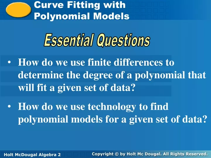
1. Curve Fitting with Polynomial Models Essential Questions • How do we use finite differences to determine the degree of a polynomial that will fit a given set of data? • How do we use technology to find polynomial models for a given set of data? Holt McDougal Algebra 2 Holt Algebra 2

2. The table shows the closing value of a stock index on the first day of trading for various years. To create a mathematical model for the data, you will need to determine what type of function is most appropriate. In Lesson 12-2, you learned that a set of data that has constant second differences can be modeled by a quadratic function. Finite difference can be used to identify the degree of any polynomial data.

4. Using Finite Differences to Determine Degree Use finite differences to determine the degree of the polynomial that best describes the data. The x-values increase by a constant 2. Find the differences of the y-values. 1. First differences: 6.3 4 2.2 0.9 0.1 Not constant Second differences: –2.3 –1.8 –1.3 –0.8 Not constant Third differences: 0.5 0.5 0.5 Constant The third differences are constant. A cubic polynomial best describes the data.

5. Using Finite Differences to Determine Degree Use finite differences to determine the degree of the polynomial that best describes the data. The x-values increase by a constant 3. Find the differences of the y-values. 2. First differences: 25 10 15 37 73 Not constant Second differences: –15 5 22 36 Not constant Third differences: 20 17 14 Not constant Fourth differences: – 3 – 3 Constant The fourth differences are constant. A quartic polynomial best describes the data.

6. Using Finite Differences to Determine Degree Use finite differences to determine the degree of the polynomial that best describes the data. The x-values increase by a constant 3. Find the differences of the y-values. 3. First differences: 20 6 0 2 12 Not constant Second differences: –14 –6 2 10 Not constant Third differences: 8 8 8 Constant The third differences are constant. A cubic polynomial best describes the data.

7. Once you have determined the degree of the polynomial that best describes the data, you can use your calculator to create the function.

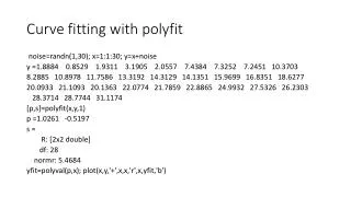
8. Using Finite Differences to Write a Function The table below shows the population of a city from 1960 to 2000. Write a polynomial function for the data. Step 1 Find the finite differences of the y-values. First differences: 918 981 1664 2982 Second differences: 63 683 1318 Third differences: 620 635 Close The third differences are constant. A cubic polynomial best describes the data.

9. Using Finite Differences to Write a Function The table below shows the population of a city from 1960 to 2000. Write a polynomial function for the data. Step 1 Find the finite differences of the y-values. Step 2 Use the cubic regression feature on your calculator. f(x) ≈ 0.10x3 – 2.84x2 + 109.84x + 4266.79

10. Using Finite Differences to Write a Function The table below shows the gas consumption of a compact car driven a constant distance at various speed. Write a polynomial function for the data. Step 1 Find the finite differences of the y-values. First differences: 1.2 0.2 -0.2 0.4 1.6 3.6 6.4 Second differences: -1 -0.4 0.6 1.2 2 2.8 Third differences: 0.6 1 0.6 0.8 0.8 Close The third differences are constant. A cubic polynomial best describes the data.

11. Using Finite Differences to Write a Function The table below shows the gas consumption of a compact car driven a constant distance at various speed. Write a polynomial function for the data. Step 1 Find the finite differences of the y-values. Step 2 Use the cubic regression feature on your calculator. f(x) ≈ 0.001x3 – 0.113x2 + 4.134x – 24.867

12. Lesson 15.1 Practice A