Download
1 / 9
90 likes | 261 Views
Curve fitting with polyfit. noise= randn (1,30); x=1:1:30; y= x+noise y =1.8884 0.8529 1.9311 3.1905 2.0557 7.4384 7.3252 7.2451 10.3703 8.2885 10.8978 11.7586 13.3192 14.3129 14.1351 15.9699 16.8351 18.6277

E N D
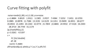
Curve fitting with polyfit noise=randn(1,30); x=1:1:30; y=x+noise y =1.8884 0.8529 1.9311 3.1905 2.0557 7.4384 7.3252 7.2451 10.3703 8.2885 10.8978 11.7586 13.3192 14.3129 14.1351 15.9699 16.8351 18.6277 20.0933 21.1093 20.1363 22.0774 21.7859 22.8865 24.9932 27.5326 26.2303 28.3714 28.7744 31.1174 [p,s]=polyfit(x,y,1) p =1.0261 -0.5197 s = R: [2x2 double] df: 28 normr: 5.4684 yfit=polyval(p,x); plot(x,y,'+',x,x,'r',x,yfit,'b')
Comparison with data and fit shown in class From class: p=0.9970 0.5981 Now: p =1.0261 -0.5197
Wrong function rather than noise yq=x+0.01*x.^2 1.0100 2.0400 3.0900 4.1600 5.2500 6.3600 7.4900 8.6400 9.8100 11.0000 12.2100 13.4400 14.6900 15.9600 17.2500 18.5600 19.8900 21.2400 22.6100 24.0000 25.4100 26.8400 28.2900 29.7600 31.2500 32.7600 34.2900 35.8400 37.4100 39.0000 >> [p,s]=polyfit(x,yq,1) p = 1.3100 -1.6533 s = R: [2x2 double] df: 28 normr: 3.6640 yqfit=polyval(p,x); plot(x,yq,'+',x,yqfit,'r') .
Using regress instead (noisy data) xx=[ones(30,1),x']; [b,bint]=regress(y',xx) b =-0.5197 1.0261 bint =-1.3124 0.2730 0.9815 1.0708 [b,bint,r,rint,stats] = regress(y',xx); stats stats =(R,the F statistic and its p value, estimate of the error variance.) 1.0e+03 * 0.0010 2.2158 0.0000 0.0011 sighat=sqrt(stats(4)) =1.0334
Residuals and cross validation errors xprimex=xx'*xx xprimex = 30 465 465 9455 E=xx*inv(xprimex)*xx'; r‘= 1.3820 -0.6796 -0.6275 -0.3942 -2.5551 1.8014 0.6621 -0.4441 1.6550 -1.4529 0.1302 -0.0351 0.49950.4670 -0.7368 0.0719 -0.0891 0.6774 1.1169 1.1068 -0.8923 0.0226 -1.2949 -1.2204 -0.1399 1.3735 -0.9549 0.1600 -0.4631 0.8538 rcross=r'./(1-diag(E)') 1.5828 -0.7674 -0.6995 -0.4343 -2.7846 1.9443 0.7085 -0.4716 1.7460 -1.5242 0.1360 -0.0365 0.51820.4836 -0.7623 0.0744 -0.0922 0.7028 1.1619 1.1557 -0.9361 0.0239 -1.3752 -1.3060 -0.1510 1.4968 -1.0519 0.1783 -0.5229 0.9778
Regress for wrong function >> [b,bint,r,rint,stats] = regress(yq',xx); b = -1.6533 1.3100 bint = -2.1845 -1.1222 1.2801 1.3399 stats = 1.0e+03 * 0.0010 8.0442 0.0000 0.0005 sighat=sqrt(stats(4))=0.6924
Corresponding residuals and cross validation “errors” r' 1.3533 1.0733 0.8133 0.5733 0.3533 0.1533 -0.0267 -0.1867 -0.3267 -0.4467 -0.5467 -0.6267 -0.6867 -0.7267 -0.7467 -0.7467 -0.7267 -0.6867 -0.6267 -0.5467 -0.4467 -0.3267 -0.1867 -0.0267 0.1533 0.3533 0.5733 0.8133 1.0733 1.3533 rcross=r'./(1-diag(E)') 1.5500 1.2120 0.9066 0.6315 0.3851 0.1655 -0.0285 -0.1982 -0.3446 -0.4686 -0.5708 -0.6520 -0.7124 -0.7525 -0.7725 -0.7725 -0.7525 -0.7124 -0.6520 -0.5708 -0.4686 -0.3446 -0.1982 -0.0285 0.1655 0.3851 0.6315 0.9066 1.2120 1.5500
Prediction variance (noisy data) • Formula from lecture • Check that at data points predvar=sighat*sqrt(diag(E))' 0.3681 0.3496 0.3314 0.3138 0.2966 0.2802 0.2644 0.2497 0.2360 0.2235 0.2127 0.2035 0.1964 0.1915 0.1890 0.1890 0.1915 0.1964 0.2035 0.2127 0.2235 0.2360 0.2497 0.2644 0.2802 0.2966 0.3138 0.3314 0.3496 0.3681 yfit= 0.5064 1.5325 2.5586 3.5848 4.6109 5.6370 6.6631 7.6892 8.7153 9.7414 10.7675 11.7936 12.8197 13.8458 14.8720 15.8981 16.9242 17.9503 18.9764 20.0025 21.0286 22.0547 23.0808 24.1069 25.1330 26.1592 27.1853 28.2114 29.2375 30.2636
For wrong function predvar=sighat*sqrt(diag(E))' predvar= 0.2466 0.2342 0.2221 0.2102 0.1988 0.1877 0.1772 0.1673 0.1581 0.1498 0.1425 0.1364 0.1316 0.1283 0.1266 0.1266 0.1283 0.1316 0.1364 0.1425 0.1498 0.1581 0.1673 0.1772 0.1877 0.1988 0.2102 0.2221 0.2342 0.2466 >> r' 1.3533 1.0733 0.8133 0.5733 0.3533 0.1533 -0.0267 -0.1867 -0.3267 -0.4467 -0.5467 -0.6267 -0.6867 -0.7267 -0.7467 -0.7467 -0.7267 -0.6867 -0.6267 -0.5467 -0.4467 -0.3267 -0.1867 -0.0267 0.1533 0.3533 0.5733 0.8133 1.0733 1.3533 >>