Download
1 / 23
240 likes | 384 Views
Chapter 5. The Duality Theorem. Given an LP, we define another LP derived from the same data, but with different structure. This LP is called the dual problem ( 쌍대문제 ).

E N D
Chapter 5. The Duality Theorem • Given an LP, we define another LP derived from the same data, but with different structure. This LP is called the dual problem (쌍대문제). • The main purpose to consider dual is to obtain an upper bound (estimate) on the optimal objective value of the given LP without solving it to optimality. Also dual problem provides optimality conditions of a solution x* for a LP and help to understand the behavior of the simplex method. Very important concept to understand the properties of the LP and the simplex method.
Approach to find optimal value of an opt. problem (max form): Find lower bound and upper bound so that for optimal value , we have • Lower bound : usually obtained from a feasible solution. If x* is a feasible solution to LP, c’x* provides a lower bound. • Upper bound : usually obtained by solving a relaxation of the problem or by finding a feasible solution to a dual problem. ex)linear programming relaxation of an integer program: Given IP, max c’x, Ax b, x 0 and integer, consider the linear programming relaxation, max c’x, Ax b, x 0. Let z* be the optimal value of IP and z’ be the optimal value of LP relaxation. Then z* z’. ( Let x* be the optimal solution of IP. Then x* is a feasible solution of LP relaxation. So there may exist a feasible solution to LP which provides better objective value)
(continued) Dual of the LP problem : Let y be a feasible solution to the dual problem. Then the dual objective value provided by y gives an upper bound on the optimal LP objective value. (study in Chapter 5.) • If the lower and upper bound are the same, we know that z* is optimal value. We may need to find the optimal solution additionally, but the optimal value is found. • Although the lower and upper bound may not be the same, from the gap (= upper bound – lower bound), we can estimate the quality of the solution we have.
Taking nonnegative linear combination of inequality constraints: Consider two constraints and …. (1’) In vector notation : If we multiply scalars y1 0 to the 1st constraint and y2 0 to the 2nd constraint and add the l.h.s. and r.h.s. respectively, we get ….. (2’) In vector notation, • Any vector that satisfies (1’) also satisfies (2’), but converse is not true. Moreover, the coefficient vector in l.h.s. of (2’) is obtained by taking the nonnegative linear combination of the coefficient vectors in (1’)
x2 2x1+x24 y1(1, 2)+y2(2, 1), y1, y2 0 x1+2x23 (1, 2) (2, 1) (5/3, 2/3) (y1a1’+y2a2’)x (3y1+4y2) x1 (0, 0)
ex) Lower bound : consider feasible solution (0, 0, 1, 0) z* 5 (3, 0, 2, 0) z* 22 Upper bound : consider inequality obtained by multiplying 0 to the 1st , 1 to the 2nd, and 1 to the 3rd constraints and add the l.h.s. and r.h.s. respectively …… (1)
Since we multiplied nonnegative numbers, any vector that satisfies the three constraints (including feasible solutions to the LP) also satisfies (1). Hence any feasible solution to LP, which satisfies the three constraints and nonnegativity, also satisfies (1). • Note that all the points satisfying 4x1 + 3x2 + 6x3 + 3x4 58 do not necessarily satisfy the three constraints in LP. • Further, any feasible solution to the LP must satisfy ( 58) since any feasible solution must satisfy nonnegativity constraints on the variables and the coefficients in the second expression is greater than or equal to the corresponding coefficients in the first expression. So 58 is an upper bound on the optimal value of the LP.
Now, we may use nonnegative weights yi for each constraint. In vector notation, Objective function of the LP is
Hence as long as the nonnegative weights yi satisfy we can use as an upper bound on optimal value. • To find more accurate upper bound (smallest upper bound), we want to solve • Dual problem obtained. Note that the objective value of any feasible solution to the dual problem provides an upper bound on the optimal value of the given LP.
General form P: primal problem, D: dual problem subject to (P) (D) subject to
Thm: (Weak duality relation) Suppose (x1, …, xn) is a feasible solution to the primal problem (P) and (y1, …, ym) is a feasible solution to the dual problem, then pf) • Cor: If we can find a feasible x* to (P) and a feasible y* to (D) such that , then x* is an optimal solution to (P) and y* is an optimal solution to (D). pf) For all feasible solution x to (P), we have Similarly, for all feasible y to (D), we have
[Strong Duality Theorem] If (P) has an optimal solution (x1*, …, xn* ), then (D) also has an optimal solution, say (y1*, …, ym* ), and (i.e., no duality gap, dual optimal value – primal optimal value = 0) Note that strong duality theorem says that if (P) has an optimal solution, the dual (D) is neither unbounded nor infeasible, but always has an optimal solution.
Idea of proof: Read the optimal solution of the dual problem from the coefficients of the slack variables in the z-row from the optimal dictionary (tableau). ex) Note that the dual variables y1, y2, y3 matches naturally with slack variables x5, x6, x7. For example x5 is slack variable for the first constraint and y1 is dual variable for the first constraint, and so on.
At optimality, the tableau looks In the z-row of the tableau, the coefficients of the slack variables are –11 for x5, 0 for x6, -6 for x7. Assigning these values with reversed signs to the corresponding dual variables, we obtain desired optimal solution of the dual: y1 = 11, y2 = 0, y3 = 6.
Idea of the proof: Note that the coefficients of x5, x6, and x7 in the z-row show what numbers we multiplied to the corresponding equation and add them to the z-row in the elementary row operations (net effect of many row operations) ex) Suppose we performed row operations (row2) 2*(row 1) +(row 2), then ( z-row) 3*(row 2) + (z-row). The net effect in z-row is adding 6*(row 1) + 3*(row 2) to the z-row and the scalar we multiplied can be read from the coefficients of x5 and x6 in the z-row.
(ex-continued) (row 1)2 + (row 2)
(ex-continued) (row 2) 3 + z-row
Example – Initial tableau Optimal tableau
Let yi be the scalar we multiplied to the i-th row and add to the z-row in the net effect. Then the coefficient of slack variables in the z-row represent the yi values we multiplied to the i-th row for i = 1, … ,m. Also the coefficients of structural variables in the z-row are given as Now in the optimal tableau, all the coefficients in the z-row are 0, which implies If we take – yi as a dual solution, they are dual feasible.
Also the constant term in the z-row gives the value So it is the negative of the dual objective valueof the dual solution (-yi ), i = 1, ,,, , m Note that the constant term in the z-row also gives the negative of the objective value of the current primal feasible solution. So we have found a feasible dual solution which gives the same dual objective value as the current primal feasible solution. From previous Corollary, the dual solution and the primal solution are optimal to the dual and the primal problem, respectively. It is the idea of the proof.
pf of strong duality theorem) Suppose we introduce slack variables and solve the LP by simplex and obtain optimal dictionary with Let We claim that yi*, i = 1, … , m is an optimal dual solution, i.e. it satisfies dual constraints and This equation must be satisfied by any x that satisfies the dictionary (excluding the nonnegativity constraints) since the set of feasible solutions does not change for any dictionary.
since any feasible solution to dictionary should satisfy this. Now this equation should hold for all feasible solutions to the dictionary. From the initial dictionary, we know that any feasible solution to the dictionary can be obtained by assigning arbitrary values to x1, … , xn and setting xn+i = bi - j=1n aijxj , ( i = 1, … , m). Use these solutions. Note that, in the above equation, the variables xn+i do not appear. So it must hold for any choices of xj , j = 1, … , n.
Equality must hold for all choices of x1, …, xn. Hence Hence y* is dual feasible. Also we have that Since yi*, i = 1, … , m is an optimal dual solution and