Download
1 / 35
350 likes | 378 Views
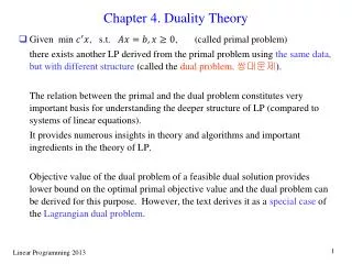
Chapter 4. Duality Theory. Given min c’x, s.t. Ax = b, x 0, (called primal problem) there exists another LP derived from the primal problem using the same data, but with different structure (called the dual problem, 쌍대문제 ).

E N D
Chapter 4. Duality Theory • Given min c’x, s.t. Ax = b, x 0, (called primal problem) there exists another LP derived from the primal problem using the same data, but with different structure (called the dual problem, 쌍대문제). The relation between the primal and the dual problem constitutes very important basis for understanding the deeper structure of LP (compared to systems of linear equations). It provides numerous insights in theory and algorithms and important ingredients in the theory of LP. Objective value of the dual problem of a feasible dual solution provides lower bound on the optimal primal objective value and the dual problem can be derived for this purpose. However, the text derives it as a special case of the Lagrangian dual problem.
Given min c’x, s.t. Ax = b, x 0, consider a relaxed problem in which the constraints Ax = b is eliminated and instead included in the objective with penalty p’(b-Ax), where p is a price vector of the same dimension as b. Lagrangian function : L(x, p) = c’x + p’(b – Ax) The problem becomes min L(x, p) = c’x + p’(b – Ax) s.t. x 0 Optimal value of this problem for fixed p Rm is denoted as g(p). Suppose x* is optimal solution to the LP, then g(p) = minx 0 [ c’x + p’(b – Ax) ] c’x* + p’(b – Ax*) = c’x* since x* is a feasible solution to LP. g(p) gives alower bound on the optimal value of the LP. Want close lower bound.
Lagrangian dual problem : max g(p) s.t. no constraints on p ,where g(p) = minx 0 [ c’x + p’(b – Ax) ] • g(p) = minx 0 [ c’x + p’(b – Ax) ] = p’b + minx 0 ( c’ – p’A )x minx 0 ( c’ – p’A )x = 0, if c’ – p’A 0 = - , otherwise Hence the dual problem is max p’b s.t. p’A c’
Remark : (1) If LP has inequality constraints Ax b Ax – s = b, s 0 [ A : -I ] [ x’ : s’ ]’ = b, x, s 0 dual constraints are p’[ A : -I ] [ c’ : 0’ ] p’A c’, p 0 Or the dual can be derived directly min c’x, s.t. Ax b, x 0 L( x, p) = c’x + p’(b – Ax) ( Let p 0 ) g(p) = minx 0 [ c’x + p’(b – Ax) ] c’x* + p’(b – Ax*) c’x* max g(p) = p’b + minx 0 ( c’ – p’A )x, s.t. p 0 min x 0 ( c’ – p’A )x = 0, if c’ – p’A 0 = - , otherwise Hence the dual problem is max p’b, s.t. p’A c’, p 0
(2) If x are free variables, then minx ( c’ – p’A )x = 0, if c’ – p’A = 0 = -, otherwise dual constraints are p’A = c’
Table 4.1 : Relation between primal and dual variables and constraints • Dual of a maximization problem can be obtained by converting it into an equivalent min problem, and then take its dual.
Vector notation min c’x max p’b s.t. Ax = b s.t. p’A c’ x 0 min c’x max p’b s.t. Ax b s.t. p’A = c’ p 0 • Thm 4.1 : If we transform the dual into an equivalent minimization problem and then form its dual, we obtain a problem equivalent to the original problem. ( the dual of the dual is primal, involution property) For simplicity, we call the min form as primal and max form as dual. But any form can be considered as primal and the corresponding dual can be defined.
(Ex 4.1) Dual Dual
Ex 4.2 : Duals of equivalent LP’s are equivalent. min c’x max p’b s.t. Ax b s.t. p 0 x free p’A = c’ min c’x + 0’s max p’b s.t. Ax – s = b s.t. p free x free, s 0 p’A = c’ -p 0 min c’x+ - c’x- max p’b s.t. Ax+ - Ax- b s.t. p 0 x+ 0 p’A c’ x- 0 -p’A -c’
Ex 4.3: Redundant equation can be ignored. Consider min c’x max p’b s.t. Ax = b (feasible) s.t. p’A c’ x 0
Thm 4.2 : If we use the following transformations, the corresponding duals are equivalent, i. e., they are either both infeasible or they have the same optimal cost. (a) free variable difference of two nonnegative variables (b) inequality equality by using nonnegative slack var. (c) If LP in standard form (feasible) has redundant equality constraints, eliminate them.
4.3 The duality theorem • Thm 4.3 : ( Weak duality ) If x is feasible to primal, p is feasible to dual, then p’b c’x. pf) Let ui = pi ( ai’x – bi ), vj = ( cj – p’Aj ) xj , If x, p feasible to P and D respectively, then ui , vj 0 i, j i ui = p’(Ax – b) = p’Ax – p’b j vj = c’x – p’Ax 0 i ui + j vj = c’x – p’b p’b c’x • Cor 4.1 : If any one of primal, dual is unbounded the other infeasible • Cor 4.2 : If x, p feasible and c’x = p’b, then x, p optimal pf) c’x = p’b c’y for all primal feasible y. Hence x is optimal to the primal problem. Similarly for p.
Thm 4.4 : (Strong duality) If a LP has an optimal solution, so does its dual, and the respective optimal costs are equal. pf) Get optimal dual solution from the optimal basis. Suppose have min c’x, Ax = b, x 0, A full row rank, and this LP has optimal solution. Use simplex to find optimal basis B with B-1b 0, c’ – cB’B-1A 0’ Let p’ = cB’B-1, then p’A c’ p’ dual feasible Also p’b = cB’B-1b = cB’xB = c’x, hence p’ optimal dual solution and c’x = p’b For general LP, convert it to standard LP with full row rank and apply the result, then convert the dual to the dual for the original LP.
1 D1 Duals of equivalent problems are equivalent Equivalent 2 D2 Duality for standard form problems Fig 4.1 : Proof of the duality theorem for general LP
(D) • Table 4.2 : different possibilities for the primal and the dual (P)
Note: (1) Later, we will show strong duality without using simplex method. (see example 4.4 later) (2) Optimal dual solution provides “certificate of optimality” certificate of optimality is (short) information that can be used to check the optimality of a given solution in polynomial time. ( Two view points : 1. Finding the optimal solution. 2. Proving that a given solution is optimal. For computational complexity of a problem, the two view points usually give the same complexity (though not proven yet, P = NP ?). Hence, researchers were almost sure that LP can be solved in polynomial time even before the discovery of a polynomial time algorithm for LP.) (3) The nine possibilities in Table 4.2 can be used importantly in determining the status of primal or dual problem.
Thm 4.5 : (Complementary slackness) Let x and p be feasible solutions to primal and dual, then x and p are optimal solutions to the respective problems iff pi ( ai’x – bi ) = 0 for all i, ( cj – p’Aj ) xj = 0 for all j. pf) Define ui = pi ( ai’x – bi ), vj = ( cj – p’Aj ) xj Then ui , vj 0 for feasible x, p ui + vj = c’x – p’b From strong duality, if x, p optimal, then c’x = p’b Hence ui + vj = 0 ui = 0, vj = 0 i, j Conversely, if ui = vj = 0 c’x = p’b, hence optimal.
Note : (1) CS theorem provides a tool to prove the optimality of a given primal solution. Given a primal solution, we may identify a dual solution that satisfies the CS condition. If the dual solution is feasible, both x and y are feasible solutions that satisfy CS conditions, hence optimal (If nondegenerate primal solution, then the system of equations has a unique solution. See ex. 4.6). (2) CS theorem does not need that x and p be basic solutions. (3) CS theorem can be used to design algorithms for special types of LP (e.g. network problems). Also interior point alg tries to find a system of nonlinear equations similar to the CS conditions. (4) See the strict complementary slackness in exercise 4.20.
Geometric view of optimal dual solution • (P) min c’x s.t. ai’x bi , i = 1, … , m x Rn , ( assume ai’s span Rn ) (D) max p’b s.t. i pi ai = c p 0 Let I { 1, … , m }, | I | = n, such that ai, i I linearly independent. ai’x = bi , i I has unique solution xI which is a basic solution. Assume that xI is nondegenerate, i.e. ai’x bi , for i I . Let p Rm be dual vector.
The conditions that xI and p are optimal are (a) ai’xI bi, i ( primal feasibility ) (b) pi = 0, i I ( complementary slackness ) (c) i pi ai = c ( dual feasibility ) iI pi ai = c ( unique solution pI ) (d) p 0, ( dual feasibility )
c c a5 a3 a1 • Figure 4.3 a4 A c a1 a2 B a3 c a4 a1 a2 c C a1 a5 D a1
Figure 4.4 degenerate basic feasible solution a2 a3 c a3 a1 a2 a1 x*
4.4 Optimal dual var as marginal costs • Suppose standard LP has nondegenerate optimal b.f.s. x* and B is the optimal basis, then for small d Rm, xB = B-1(b+d) > 0. c’ – cB’B-1A 0’ not affected, hence B remains optimal basis. Objective value is cB’B-1(b + d) = c’x* + p’d ( p’ = cB’B-1 ) So pi is marginal cost (shadow price) of i-th requirement bi.
4.5 Dual simplex method • For standard problem, a basis B gives primal solution xB = B-1b, xN = 0 and dual solution p’ = cB’B-1 At optimal basis, have xB = B-1b 0, c’ – p’A 0 ( p’A c’) and cB’B-1b = cB’xB = p’b, hence optimal ( have primal feasible, dual feasible solutions and objective values are the same). Sometimes, it is easy to find dual feasible basis. Then, starting from a dual feasible basis, try to find the basis which satisfies the primal feasibility. (Text gives algorithm for tableau form, but revised dual simplex algorithm also possible.)
Given tableau, cj 0 for all j, xB(i) < 0 for some i B. (1) Find row l with xB(l) < 0. vi is l-th component of B-1Ai (2) For i with vi < 0, find j such that cj / | vj | = min{ i : vi < 0 }ci / | vi | (3) Perform pivot ( Aj enters, AB(l) leaves basis ) ( dual feasibility maintained)
Note : (1) row 0 row 0 + ( l-th row ) cj / | vj | ci ci + vi ( cj / | vj | ) ( ci 0 from the choice of j ) For vi > 0, add vi (nonnegative number) to row 0 ci 0 For vi < 0, have cj / | vj | ci / | vi |. Hence dual feasibility maintained. - cB’B-1b - cB’B-1b + (xB(l) cj ) / | vj | = - (cB’B-1b – (xB(l) cj ) / | vj | ) Objective value increases by – (xB(l) cj ) / | vj | 0. ( note that xB(l) < 0, cj 0 ) If cj> 0, objective value strictly increases.
(2) If cj > 0, j N in all iterations, objective value strictly increases, hence finite termination. (need lexicographic pivoting rule for general case) At termination case a) B-1b 0, optimal solution. case b) entries v1, … , vn of row l are all 0, then dual is unbounded. Hence primal is infeasible. ( reasoning : (1) Find unbounded dual solution. Let p’ = cB’B-1 be the current dual feasible solution ( p’A c’). Suppose xB(l) < 0. Let q’ = - el’B-1 (negative of l-th row of B-1), then q’b = - el’B-1b > 0 and q’A = - el’B-1A 0. Hence ( p + q)’b as and p + q is dual feas. (2) Current row l : xB(l) = i vixi Since vi 0, and xi 0 for feasibility, but xB(l) < 0 no feasible solution to primal exists hence dual unbounded. )
The geometry of the dual simplex method • For standard LP, a basis B gives a basic solution (not necessarily feasible) xB = B-1b, xN = 0. The same basis provides a dual solution by p’AB(i) = cB(i) , i = 1, … , m, i. e. p’B = cB’. The dual solution p’ is dual feasible if c’ – p’A 0. So, in the dual simplex, we search for dual b.f.s. while corresponding primal basic solutions are infeasible until primal feasibility (hence optimality) is attained. ( see Figure 4.5 ) • See example 4.9 for the cases when degeneracy exists
4.6 Farkas’ lemma and linear inequalities • Thm 4.6 : Exactly one of the following holds: (a) There exists some x 0 such that Ax = b (b) There exists some p such that p’A 0 and p’b < 0 (Note that we used (I) y’A = c’, y 0 (II) Ax 0, c’x > 0 earlier. Rows of A are considered as generators of a cone. But, here, columns of A are considered as generators of a cone.) pf) not both : p’Ax = p’b 0 ( i.e. one holds the other not hold) Text shows (a) ~(b) which is equivalent to (b) ~(a) ~(a) (b) : Consider (P) max 0’x (D) min p’b Ax = b p’A 0’ x 0 ~(a) primal infeasible dual infeasible or unbounded but p = 0 is dual feasible dual unbounded p with p’A 0’ and p’b < 0
Other expression for Farkas’ lemma. Cor 4.3 ) Suppose that any vector p satisfying p’Ai 0, i = 1, … , n also satisfy p’b 0. Then x 0 such that Ax = b. • See ‘Applications of Farkas’ lemma to asset pricing’ and separating hyperplane theorem used for proving Farkas’ lemma.
The duality theorem revisited • Proving strong duality using Farkas’ lemma (not using simplex method as earlier) (P) min c’x (D) max p’b s.t. Ax b p’A = c’ p 0 Suppose x* optimal to (P). Let I = { i : ai’x* = bi } Then d that satisfies ai’d 0, i I, must satisfy c’d 0 ( i. e. ai’d 0, i I, c’d < 0 infeasible ) ( Note that above statement is nothing but saying, if x* optimal, then there does not exists a descent and feasible direction at x* . Necessary condition for optimality of x* )
(continued) Otherwise, let y = x* + d Then ai’ ( x* + d ) = ai’x* + ai’d ai’x* = bi , i I ai’ ( x* + d ) = ai’x* + ai’d > bi , for small > 0, i I Hence y feasible for small and c’y = c’x* + c’d < c’x* Contradiction to optimality of x*. By Farkas’, pi 0, i I such that c = iI piai. Let pi = 0 for i I p 0 such that p’A = c’ and p’b = iI pibi = iI piai’x* = c’x* By weak duality, p is optimal dual solution.
a3 • Figure 4.2 strong duality theorem a2 a1 c p2a2 p1a1 { ai’d0, i I } x* c’d < 0