Download
1 / 17
270 likes | 643 Views
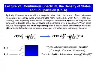
Lecture 20. Continuous Spectrum, the Density of States (Ch. 7), and Equipartition (Ch. 6).

E N D
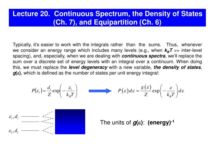
Lecture 20. Continuous Spectrum, the Density of States (Ch. 7), and Equipartition (Ch. 6) Typically, it’s easier to work with the integrals rather than the sums. Thus, whenever we consider an energy range which includes many levels (e.g., when kBT >> inter-level spacing), and, especially, when we are dealing with continuous spectra, we’ll replace the sum over a discrete set of energy levels with an integral over a continuum. When doing this, we must replace the level degeneracy with a new variable, the density of states, g(), which is defined as the number of states per unit energy integral: The units of g(): (energy)-1
The density of states, g(), is the number of states per unit energy The Density of States Page 279, Ch. 7 Let’s consider G() - the number of states per unit volume with energy less than (for a one- and two-dimensional cases, it will be the number of states with energy less than per unit length or area, respectively). Then the density of states is its derivative: The number of states per unit volume in the energy range – +d : The probability that one of these states is occupied: The probability that the particle has an energy between and+d : Since the partition function is
The Density of States for a Single Free Particle in 1D The energy spectrum for the translational motion of a molecule in free space is continuous. We will use a trick that is common in quantum mechanics: assume that a particle is in a large box (energy quantization) with zero potential energy (total energy= kin. energy). At the end of the calculation, we’ll allow the size of the box to become infinite, so that the separation of the levels tends to zero. For any macroscopic L, the energy levels are very close to each other (E ~ 1/L2), and the “continuous” description works well. For a quantum particle confined in a 1D “box”, the stationary solutions of Schrödinger equation are the standing waves with the wavelengths: the wave number where The momentum in each of these states: k - the energy (the non-relativistic case) In the “k” (i.e., momentum) space, the states are equidistantly positioned (in contrast to the “energy” space).
The Density of States for a Single Free Particle in 1D (cont.) The total number of states with the wave numbers < k is: G(k) - the number of states additional degeneracy of the states (2s+1) because of spin [e.g., forelectrons 2s+1=2] g() 1D
2D g() 3D The Density of States for a Particle in 2D and 3D ky For quantum particles confined in a 2D “box” (e.g., electrons in FET): 2D k kx g() # states within ¼ of a circle of radius k - does not depend on 3D kz kx ky Thus, for 3D electrons (2s+1=2):
Partition Function of a Free Particle in Three Dimensions Z1 – a reminder that this is the partition function for a single particle The mean energy can be found without evaluating the integral: The numerator can be integrated by parts: (the integrand vanishes at both limits) - in agreement with the equipartition theorem
The Partition Function of a Free Particle (cont.) (assume that s=0) - the quantum volume and density For unit volume (V=1): the quantum length, coincides [within a factor of ()1/2 ] with the de Broglie length of a particle whose kinetic energy is kBT. VQis the volume of a box in which the ground state energy would be approximately equal to the thermal energy, and only the lowest few quantum states would be significantly populated. When V VQ, the continuous approximation breaks down and we must take quantization of the states into account. We also need to consider quantum statistics (fermions and bosons)!
There is nothing in the derivation of the partition function or the Boltzmann factor that restricts it to a microsystem. However, it is often convenient to express the partition function of a combined macrosystem in terms of the single-particle partition function. We restrict ourselves to the case of non-interacting particles (the model of ideal gas). Partition Functions for Distinguishable Particles Recall the analogy between and Z: For a microcanonical ensemble, we know the answer for total: How about the canonical ensemble? For two non-interacting particles, Etotal =E1+E2 : distinguishable all the states for the composite system non-interacting distinguishable particles Example: two non-interacting distinguishable two-state particles, the states 0 and : The partition function for a single particle: The states of this two-particle system are: (0,0), (,), (,0), (0,) - distinguishable
1 2 = 2 1 Partition Functions for Indistinguishable Particles (Low Density Limit) If the particles are indistinguishable, the equation should be modified. Recall the multiplicity for IG: If the states (,0) and (0,) of a system of two classical particles are indistinguishable: (For the quantumindistinguishable particles, there would be three microstates if the particles were bosons [(0,0), (0,), (,)] and one microstate [(0,)] if the particles were fermions). For two indistinguishable particles: Exceptions: the microstates where the particles are in the same state. If we consider particles in the phase space whose volume is the product of accessible volumes in the coordinate space and momentum space (e.g., an ideal gas), the states with the same position and momentum are very rare (unless the density is extremely high) For a low-densitysystem of classical indistinguishable particles:
Z and Thermodynamic Properties of an Ideal Gas The partition function for an ideal gas: Note that the derivation of Z for an ideal gas was much easier than that for : we are not constrained by the energy conservation! - the “pressure” equation of state (“ideal gas” law) - the Sackur-Tetrode equation - the “energy” equation of state
The Equipartition Theorem (continuous spectrum) Equipartition Theorem: At temperature T, the average energy of any quadratic degree of freedom is ½kBT. E(q) We’ll consider a “one-dimensional” system with just one degree of freedom: q – a continuous variable, but we “discretize” it by considering small and countable q’s: q q The partition function for this system: New variable: exp(-x2) The average energy: x Again, this result is valid only if the degree of freedom is “quadratic” (the limit of high temperatures, when the spacing between the energy levels of an individual system is << kBT).
Equipartition Theorem and a Quantum Oscillator Classical oscillator: Quantum oscillator: the equipartition function: the average energy of the oscillator: the limit of high T: (the ground state is by far the most probable state) the limit of low T: the assumption of a continuous energy spectrum was violated
The Maxwell Speed Distribution (ideal gas) The probability that a molecule has an energy between and +d is: g() P() = 0 0 0 Now let’s look at the speed distribution for these particles: The probability to find a particle with the speed between v and v+dv,irrespective of the direction of its velocity, is the same as that finding it between and +d where d= mvdv: Maxwell distribution Note that Planck’s constant has vanished from the equation – it is a classical result.
P(v) v The Maxwell Speed Distribution (cont.) vy The structure of this equation is transparent: the Boltzmann factor is multiplied by the number of states between v and v+dv. The constant can be found from the normalization: v vx vz energy distribution, N – the total # of particles speed distribution P(vx) distribution for the projection of velocity, vx vx
The Characteristic Values of Speed Because Maxwell distribution is skewed (not symmetric in v), the root mean square speed is not equal to the most probable speed: P(v) The root-mean-square speed is proportional to the square root of the average energy: v The most probable speed: The average speed:
Problem (Maxwell distr.) Consider a mixture of Hydrogen and Helium at T=300 K. Find the speed at which the Maxwell distributions for these gases have the same value.
Problem (final 2005, MB speed distribution) • Consider an ideal gas of atoms with mass m at temperature T. • Using the Maxwell-Boltzmann distribution for the speed v, find the corresponding distribution for the kinetic energy (don’t forget to transform dv into d). • Find the most probable value of the kinetic energy. • Does this value of energy correspond to the most probable value of speed? Explain. (a) (b) doesn’t correspond (c) the most probable value of speed the kin. energy that corresponds to the most probable value of speed