Download
1 / 18
180 likes | 490 Views
Rossby wave propagation. Propagation…. Three basic concepts: Propagation in the vertical Propagation in the y-z plane Propagation in the x-y plan. 3. Propagation in the x-y plane Reference back to Hoskins & Karoly (HK, 1981)

E N D
Propagation… Three basic concepts: • Propagation in the vertical • Propagation in the y-z plane • Propagation in the x-y plan
3. Propagation in the x-y plane • Reference back to Hoskins & Karoly (HK, 1981) • They extended earlier work (Grose & Hoskins (GH), 1979) which used a barotropic model on the sphere. • GH showed that flow over a simple mountain could generate a “downstream” (not necessarily zonal) response with a wavelike nature. • HK seek to extend this to include: • Baroclinic responses (via a baroclinic model) • Responses to a heat source
Propagation in the x-y plane • The model used: • Primitive equation, -coordinate, 5 levels (only!!) • Equations are linearized about a realistic basic state [U(x,y,z)] • A steady solution is assumed, so the t terms are eliminated • Eq 2.6 is the matrix form of the linearized equations (LHS is dX/dt) • Adding dissipation (D) and forcing (F) and assuming a steady solution (d/dt = 0) gives the equation before (2.8) and the solution is (2.8) by matrix inversion
Propagation in the x-y plane • In the east-west direction, structures are sine/cosine waves (wavenumber “m”) • In the north-south direction, structures are given by associated Legendre functions (Holton?) • The spectral truncation is generally J=25, which covers waves 0, 1,2,3 etc. thru 13. This is in the N-S direction. • In the E-W direction, they go out to wave 26 (or sometimes 6)
Propagation in the x-y plane • Forcing is prescribed via a heat source at a given location (balanced by cooling elsewhere to give no net heating) and with a given vertical structure • Fig 3 shows the response computed to a tropical heat source
Propagation in the x-y plane • Observation from • Wallace & Gutzler • (more later!)
Propagation in the x-y plane • Thus far we have a model (actually two) that produce patterns that look a lot like teleconnections. • How do we understand these patterns? • Hoskins & Karoly go into the theory in section 5. • The linearized equations reduce to (5.9) • (5.11) is the dispersion equation given a wave-like solution • We can define a group velocity vector as:
Propagation in the x-y plane • For a stationary wave, we set =0, and we define a rayas a line whose slope is given by cg everywhere, and which represents the direction of energy propagation. • Energy propagates along a ray with speed |cg|. • The shape of the ray is given by: • Along a ray, k remains fixed, but lcan vary. • HK define Ks2=(k2+l2), and Ks2 is given by (5.16). • So as the background wind varies (5.10), M varies, which changes Ks and thus l, the meridional wavenumber.
Propagation in the x-y plane • HK look for a solution like (5.18) and develop the equation for the meridional structure function P(y) – this is (5.19). • The solution is (5.23) via the WKB assumption. • Thus we know the amplitude of the solution along the ray. • Some background information (from James’ book): • The group velocity gives the direction and rate at which “wave action” is spread away from the source region. • James defines the “wave action density” as:
Propagation in the x-y plane • The quantity cgyA is conserved along a ray (as long as the background varies “slowly” only in y). • It can be shown that • And thus as l decreases as a wave propagates poleward, it’s amplitude increases. • Thus a relatively “small” forcing a lower latitudes can give a large response in midlatitudes.
Propagation in the x-y plane • Back to HK… • Using the relations developed, one can compute the progress of a ray as time evolves, and one can compute the wave amplitude along the ray. • Figures 14 & 15 give examples.
Propagation in the x-y plane - summary • HK solved the linearized equations to find the structure on the sphere of a Rossby wave train forced by an isolated heat source. • The results bear a strong resemblance to observed teleconnections patterns (i.e., in character). • The theory indicates that we expect rays to propagate away from the source region following a great circle, and with speed and direction and wave amplitude given in terms of basic wave and background properties (including wavenumber and the mean wind profile).
Propagation in the x-y plane - summary • Based on this work (and other studies), there is plenty of reason to believe that teleconnections owe their existence to Rossby wave trains that have propagated considerable distances around the globe. • Next – let’s look at and review some of the more prominent teleconnection patterns.