Download
1 / 30
300 likes | 452 Views
ADVENTURE IN SYNOPTIC DYNAMICS HISTORY. How can we tell when and where air is going to go up?. The diagnosis of mid-latitude vertical motions. CHAPTER 6 in Mid-latitude atmospheric dynamics. Why are we interested in vertical motions in the atmosphere?. Note that. and.

E N D
The diagnosis of mid-latitude vertical motions CHAPTER 6 in Mid-latitude atmospheric dynamics Why are we interested in vertical motions in the atmosphere?
Note that and UNDERSTANDING AGEOSTROPHIC FLOW The relationship between the ageostrophic wind and the acceleration vector Vector form of eqn. of motion Divide by f and take vertical cross product
Black arrows: acceleration vector Gray arrows: ageostrophic wind vector Ageostrophic wind and acceleration vectors in a jetstreak
Black arrows: acceleration vector Gray arrows: ageostrophic wind vector Ageostrophic wind and acceleration vectors in a trough-ridge system
Let’s only consider the geostrophic contribution to Convergence and divergence of the ageostrophic wind: two simple cases ageostrophic flow in vicinity of jetstreaks and curved flow Let’s only consider the first term
jet exit Conv Div pressure increasing under jet right exit region pressure decreasing under jet right exit region H L Geostrophic wind relationship Pressure coordinates Height coordinates This component of the ageostrophic wind is called the isallobaric wind because the ageostrophic wind flows in the direction of the gradient in the pressure tendency
jet exit Conv Div pressure increasing under jet right exit region pressure decreasing under jet right exit region H L Convergence of the near surface (ageostrophic) isallobaric wind is related to rising motion
Let’s only consider the geostrophic contribution to Convergence and divergence of the ageostrophic wind: two simple cases ageostrophic flow in vicinity of jetstreaks and curved flow Let’s only consider the second term
This ageostophic wind component is called the inertial-advective wind Let’s expand this: At black dot: Inertial advective component flows cross jet, consistent with divergence and convergence patterns in jetstreak Exit region of a jetstreak
This ageostophic wind component is called the inertial-advective wind Let’s expand this: At black dot: Inertial advective component flows in direction of geostrophic wind, consistent with supergeostrophic flow in crest of ridge Exit region of a jetstreak
Sutcliff’s (1939) expression for ageostrophic divergence Consider a surface wind Consider a wind aloft such that Consider the vertical shear vector Expand expression in orange box: and and rewrite: and note that: So we can write:
The difference between the acceleration of the wind aloft and the acceleration of the wind at the surface is related to the shear over the surface wind gradient and the rate of change of the wind shear following parcel motion. (are you rather confused??) Let’s take it apart and try to understand a simple example Examine first term on RHS:
Dashed lines: 1000-500 mb thickness (mean temperature in 1000-500 mb layer) Solid lines: Isobars Little arrows: Geostrophic wind Black arrow: Gray arrow: Difference between upper and lower level ageostrophic wind Red arrow: Shear vector Shear northward along direction of mean isentropes At center of low:
Dashed lines: 1000-500 mb thickness (mean temperature in 1000-500 mb layer) Solid lines: Isobars Little arrows: Geostrophic wind Black arrow: Gray arrow: Difference between upper and lower level ageostrophic wind Red arrow: Shear vector (black arrow) Direction of difference in ageostrophic wind between top and bottom of column gray arrow
(black arrow) Direction of difference in ageostrophic wind between top and bottom of column gray arrow Ageostrophic wind at surface at low center = 0 Ageostrophic wind aloft points south Aloft: wind diverges at D, convergences at C Low propagates toward D, or along the direction of the geostrophic shear (mean isotherms) THE SEA-LEVEL PRESSURE PERTURBATION PROPAGATES IN THE DIRECTION OF THE THERMAL WIND VECTOR
The difference between the acceleration of the wind aloft and the acceleration of the wind at the surface is related to the shear over the surface wind gradient and the rate of change of the wind shear following parcel motion. (are you rather confused??) Let’s take it apart and try to understand a second simple example Examine second term on RHS:
FRONTOGENESIS Dashed lines: 1000-500 mb thickness Thin gray arrows: Shear vector Black arrow: Gray arrow: Gray arrow is the difference in the ageostrophic flow between upper and lower troposphere Air diverges aloft on warm side of front: rising motion on warm side Air converges aloft on cold side of front: sinking motion on cold side 1939: First dynamical understanding of the effect of frontogenesis on vertical circulations about fronts
Consider the historical significance of this equation: In 1939, when Sutcliff published this result, the U.S. Military weather forecasters were just beginning to launch rawinsondes around the country. There were no computers or forecast models. This relationship allowed forecasters, from measurements of temperature at two levels and the sea level pressure field, to forecast the direction of movement of highs and lows! The relationship also allowed forecasters to diagnose where upward motion would occur by comparing the 1000-500 mb thickness patterns at two times.
The Sutcliffe Development Theorem (1949) Recall equation for ageostrophic wind and apply operator: Use the vector identity: Sutcliff reasoned that: On an f plane (f constant) the divergence Of the ageostrophic wind is related to Changes in the vertical component of vorticity …and sought to understand how vorticity may be used as a diagnostic tool to determine where divergence, and hence rising motions might occur Let’s look at Sutcliff’s reasoning…..
Divergence of ageostrophic wind related to change in vorticity Let’s start with the vorticity equation in 2D (ignoring the tilting terms) Expand total derivative Now assume 1) vorticity and horizontal winds are geostrophic 2) vertical advection of vorticity is negligible 3) relative vorticity can be neglected in divergence term Or:
Sutcliff’s idea: Consider difference in divergence between the top and bottom of an air column (say at 300 and 700 mb) is the change in thickness between two height surfaces where
Recall thickness is related To mean temperature between two levels What is a change in thickness associated with? Let’s find out by expanding total derivative Diabatic heating or cooling Thickness advection Vertical advection (adiabatic heating or cooling) Sutcliff 1) ignored diabatic cooling as small, 2) ignored vertical advection to simplify the problem 3) assumed V = Vg = mean geostrophic wind in layer
Original equation Term on far RHS Now substitute thermal wind eqn:
Expand this term, eliminating products of derivatives as small. The terms that are eliminated represent deformation, and they are therefore associated with frontogenesis Terms in yellow represent divergence of mean geostrophic wind and thermal wind Both = 0 Surviving terms in vector form:
Note that these are expressions of relative vorticity Surviving terms in vector form: Substitute:
Original equation Simplified form of term on RHS Plug it in: Reduce right hand side And finally….
Synoptic scale vertical motions: (the result of greater divergence or convergence aloft in an air column) can be diagnosed on weather maps How? Plot geopotential height field at two levels Graphically subtract them to get thermal wind vector Use same fields to determine vorticity at each level (using ) add them up and determine advection of total vorticity by thermal wind Today this all seems like too much work!!! But in 1949, the technique revolutionized synoptic meteorology
Sutcliff vertical motion at 500 mb (microbars/s) 300-700 mb thickness Vorticity term in Sutcliff equation actual vertical motion At 500 mb (microbars/s)