Summary Table of Influence Procedures for a Single Sample (I)

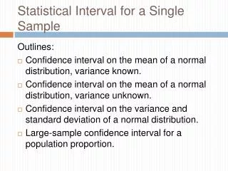
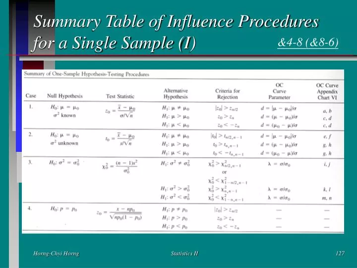
1. Summary Table of Influence Procedures for a Single Sample (I) &4-8 (&8-6) Statistics II

2. Summary Table of Influence Procedures for a Single Sample (II) Statistics II

3. Testing for Goodness of Fit &4-9 (&8-7) • In general, we do not know the underlying distribution of the population, and we wish to test the hypothesis that a particular distribution will be satisfactory as a population model. • Probability Plotting can only be used for examining whether a population is normal distributed. • Histogram Plotting and others can only be used to guess the possible underlying distribution type. Statistics II

4. Goodness-of-Fit Test (I) • A random sample of size n from a population whose probability distribution is unknown. • These n observations are arranged in a frequency histogram, having k bins or class intervals. • Let Oi be the observed frequency in the ith class interval, and Ei be the expected frequency in the ith class interval from the hypothesized probability distribution, the test statistics is Statistics II

5. Goodness-of-Fit Test (II) • If the population follows the hypothesized distribution, X02 has approximately a chi-square distribution with k-p-1 d.f., where p represents the number of parameters of the hypothesized distribution estimated by sample statistics. • That is, • Reject the hypothesis if Statistics II

6. Goodness-of-Fit Test (III) • Class intervals are not required to be equal width. • The minimum value of expected frequency can not be to small. 3, 4, and 5 are ideal minimum values. • When the minimum value of expected frequency is too small, we can combine this class interval with its neighborhood class intervals. In this case, k would be reduced by one. Statistics II

7. Example 8-18The number of defects in printed circuit boards is hypothesized to follow a Poisson distribution. A random sample of size 60 printed boards has been collected, and the number of defects observed as the table below: • The only parameter in Poisson distribution is l, can be estimated by the sample mean = {0(32) + 1(15) + 2(19) + 3(4)}/60 = 0.75. Therefore, the expected frequency is: Statistics II

8. Example 8-18 (Cont.) • Since the expected frequency in the last cell is less than 3, we combine the last two cells: Statistics II

9. Example 8-18 (Cont.) 1. The variable of interest is the form of distribution of defects in printed circuit boards. 2. H0: The form of distribution of defects is Poisson H1: The form of distribution of defects is not Poisson 3. k = 3, p = 1, k-p-1 = 1 d.f. 4. At a = 0.05, we reject H0 if X20 > X20.05, 1 = 3.84 5. The test statistics is: 6. Since X20 = 2.94 < X20.05, 1 = 3.84, we are unable to reject the null hypothesis that the distribution of defects in printed circuit boards is Poisson. Statistics II

10. Contingency Table Tests (&8-8) • Example 8-20 A company has to choose among three pension plans. Management wishes to know whether the preference for plans is independent of job classification and wants to use a = 0.05. The opinions of a random sample of 500 employees are shown in Table 8-4. Statistics II

11. Contingency Table Test- The Problem Formulation (I) • There are two classifications, one has r levels and the other has c levels. (3 pension plans and 2 type of workers) • Want to know whether two methods of classification are statistically independent. (whether the preference of pension plans is independent of job classification) • The table: Statistics II

12. Contingency Table Test- The Problem Formulation (II) • Let pij be the probability that a random selected element falls in the ijth cell, given that the two classifications are independent. Then pij = uivj, where the estimator for ui and vj are • Therefore, the expected frequency of each cell is • Then, for large n, the statistic has an approximate chi-square distribution with (r-1)(c-1) d.f. Statistics II

13. Example 8-20 Statistics II

14. Statistics II