Download

1 / 55
550 likes | 626 Views
Designs for environmental monitoring. Gerry Quinn & Mick Keough, 2002 Do not copy or distribute without permission of authors. Some consistent terminology. T ime divided into two major Periods , Before and After. Within these periods are Times (e.g. years) and subdivisions of times

E N D
Designs for environmental monitoring Gerry Quinn & Mick Keough, 2002 Do not copy or distribute without permission of authors.
Some consistent terminology • Time • divided into two major Periods, Before and After. • Within these periods are Times (e.g. years) • and subdivisions of times • Spatial areas • divided into two major groups, Control and Impact • Within each group are Locations • larger spatial units • different areas in which the same kind of management • i.e., true replicates of the management activity • and subsamples within locations
Controls & Impacts • Control areas lack the management action • = Reference areas • Impacts are effects of management action
Restricted Designs CONTROL & IMPACT Control Impact BEFORE & AFTER Before After
Better Designs:Multiple controls & impacts CONTROL SITES IMPACT SITES
Williamstown Rifle Range • Replicate open (C) and closed (I) locations • Single point in time • Four harvested species • Three unharvested species • Keough et al. (1993) Cons. Biol.
km 0 1 2 Rifle Range WILLIAMSTOWN RR2 ALTONA A1 W1 RR1 W4 W3 W2 A2
Turban Snails Marine Research Group, Coastal Invertebrates of Victoria From Edgar, Australian Marine Life
WRR: early study • Three of 4 harvested species larger in protected areas • No differences in unharvested species • Power calculations for unharvested species
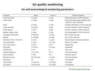
Three common models • BACI & BACIP • Stewart Oaten / Green • Beyond-BACI • Underwood • MBACI • Keough & Mapstone
1 2 3 4 5 6 BACI(P) DESIGN BEFORE IMPACT AFTER IMPACT Time CONTROL SITE IMPACT SITE
BACIP • Impact and single Control location • Sampling through time (B & A) • Times within B & A • Test is divergence of two locations after management activity • uses C-I as test measure • Only one control location of interest • does Impact change relative to standard?
Calculations in BACI design d Time Time
Impact Control Procedure • Plot values for each location through time • Calculate di = Ci - Ii for each time • Compare d values between groups (Before & After) - ANOVA or t-test. Time
BACIP: replication & power • Replicates are times within B & A • Each location represented by single value in analysis • Subsampling of locations useful to characterize each location well • Indirect effect on power • Power primarily determined by time • Needs longer sampling period, • not more frequent samples
Assumptions of BACIP • Independence of C & I • No serial correlation • Value of d at time i independent of value at time i+1 • C & I “track” well through time in absence of impact • Control is well-chosen
Choosing control locations • As similar as possible to I, except for presence of activity in question • Physically similar • Fauna & flora similar • Far enough away to be free of effects of activity
Choosing controls – a freshwater example. Within a catchment • substrate/geology/suspended load • discharge regime/stream or catchment size • riparian vegetation/zone • catchment land use/vegetation/soils • gradient • altitude/stream order/dist. from source • current speed/riffle & pool structure • spatial proximity/external variables • water quality including detritus levels • channel form/geometry
Choosing controls within a catchment • algal cover • where I'm prepared to drink the water • logistical practicality • Chance • presence of fish • aspect
Choosing controls between catchments • substrate • discharge regime/stream size • catchment land use/vegetation • riparian vegetation • gradient • geographic proximity • geomorphic forms/hydraulic habitat • altitude and aspect/temperature • water quality/geology • can't be guessed/not solvable/no answer
Steps to choosing controls • Conduct a literature review • Draw up a list of criteria ordered from most important to least • Carry out location visits • Are there sufficient control locations? • Revisit the criteria • Does this improve the number of control locations?
BACIP example: San Onofre Nuclear Generating Station (SONGS) • Seawater used in cooling system • Discharge 6000 m3/min • 1 km2/d, 3-4 m deep • Temperature raised by 10ºC • Water released through diffusers • Plume entrains 60,000 m3
Before After Control Impact 1 2 3 4 5 6 Sampling Times
Before After Control Impact 1 2 3 4 5 6 “Plots”
1 2 3 4 5 6 Factor A (Periods) Factor C (C-I) “Plots”
The linear model • Times (T) nested within Before & After (BA) • Crossed with Control-Impact (CI) • Time random, but BA and CI are fixed • DV = + BA +T(BA) + CI + BA*CI • No replication (no Times x CI interaction) • Power depends on # of times
MBACI • Multiple Control and Impact locations • Times within Before & After • Do Impact locations diverge relative to suite of Control areas? • Controls represent whole range of unmanaged areas • All available times (e.g. years) presumed to be sampled
Before After Sites Control Impact 1 2 3 4 5 6 Times 1 2 3 4 5
MBACI: linear model • Now four factors: • BA - fixed • Times within Before & After - fixed?? • CI - fixed • Sites within Control & Impact - random • DV= + BA + T(BA) + CI + S(CI) + BA*CI + CI*T(BA) + BA*S(CI) • Test BA*CI using BA*S(CI) as denominator
MBACI • Power depends on # of sites • Because test is made with BA x sites, critical assumptions are about how the BA changes occur at the “replicate” sites • Are these changes normal, homogeneous variances, etc?
MBACI: subsampling • Replicates are locations • direct effect on power • Subsamples to characterize location-time combinations • subsamples affect power by reducing L x B-A variance • “Replicate” times used only to estimate B & A conditions • affect power by reducing L x B-A variance
MBACI example - Keough & Quinn (2000) • Effect of marine protected areas in the absence of strict enforcement • Areas open to recreational harvesting for >75 y, and areas closed for 75 y, opened in 1992 • DV is mean size of a common limpet • Factor A: Harvesting • units of replication are individual reefs • Factor B (reefs) nested within factor A
Factor C: Before and After opening of shoreline • units of replication years • Factor D (years) nested within Factor C • Factors A & C fixed • nested factor B (sites) is random • nested factor D (years) is fixed
ANOVA table Source of Variation Num Den MS F P Df Df Harvesting 1 6 0.010 Before-After 1 6 0.007 H x B-A 1 6 0.015 Sites(Harvesting) 6 Res 0.119 Years(B-A) 6 Res 0.008 Sites x B-A 6 Res 0.951 Year x Harvesting 6 Res 0.714 Residual MS 31 12.593 Key test is H x B-A, which is tested using Sites x B-A. This effect is significant
Cellana tramoserica 40 I C 30 Shell Length (mm) 20 10 89 90 91 93 94 95 96 97
WRR: broken protection • Impact was opening of Rifle Range • 3 years Before • 7 years After • Additional Controls using unharvested species • Keough & Quinn (2000), Ecol. Appl
WRR broken protection • Declines in size, abundance of Cellana, Turbo, no change in less harvested species • No change in unharvested species • Power
Example 2: Liming of streams • Aim: Evaluate restoration methods for Welsh streams affected by acid rain • described by Downes et al., (2002), 8.4.1 • “Impact” would be enhancement of salmonid fish & invertebrates following raising of pH • Impacts can be good! • Control is streams with no restoration