Download
1 / 18
220 likes | 922 Views
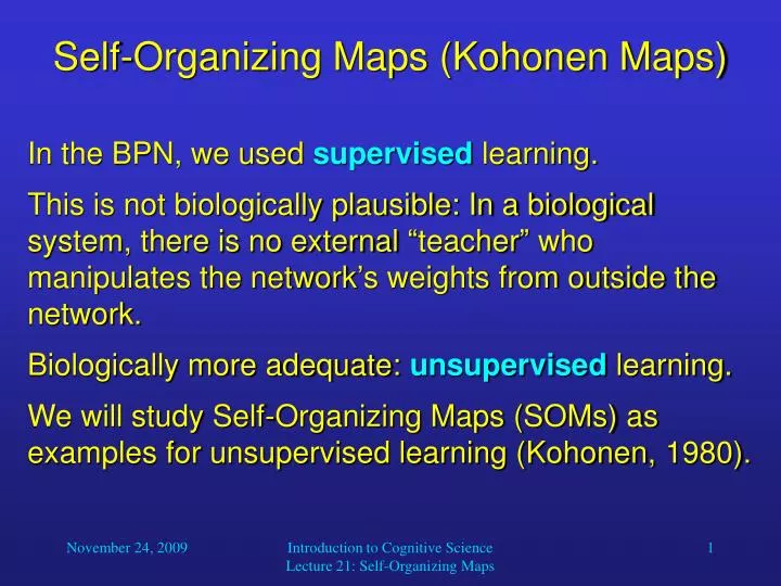
Self-Organizing Maps (Kohonen Maps). In the BPN, we used supervised learning. This is not biologically plausible: In a biological system, there is no external “teacher” who manipulates the network’s weights from outside the network. Biologically more adequate: unsupervised learning.

E N D
Self-Organizing Maps (Kohonen Maps) In the BPN, we used supervised learning. This is not biologically plausible: In a biological system, there is no external “teacher” who manipulates the network’s weights from outside the network. Biologically more adequate: unsupervised learning. We will study Self-Organizing Maps (SOMs) as examples for unsupervised learning (Kohonen, 1980). Introduction to Cognitive Science Lecture 21: Self-Organizing Maps
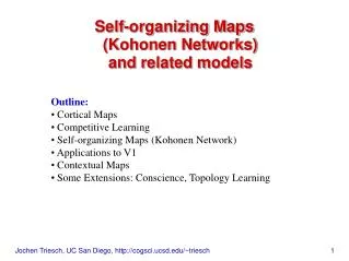
Self-Organizing Maps (Kohonen Maps) In the human cortex, multi-dimensional sensory input spaces (e.g., visual input, tactile input) are represented by two-dimensional maps. The projection from sensory inputs onto such maps is topology conserving. This means that neighboring areas in these maps represent neighboring areas in the sensory input space. For example, neighboring areas in the sensory cortex are responsible for the arm and hand regions. Introduction to Cognitive Science Lecture 21: Self-Organizing Maps
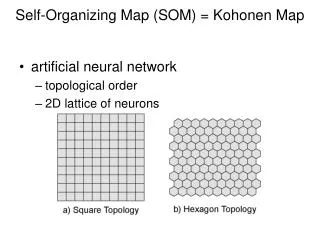
Self-Organizing Maps (Kohonen Maps) • Such topology-conserving mapping can be achieved by SOMs: • Two layers: input layer and output (map) layer • Input and output layers are completely connected. • Output neurons are interconnected within a defined neighborhood. • A topology (neighborhood relation) is defined on the output layer. Introduction to Cognitive Science Lecture 21: Self-Organizing Maps
Self-Organizing Maps (Kohonen Maps) output vector o • BPN structure: … O1 O2 O3 Om … I1 I2 In input vector x Introduction to Cognitive Science Lecture 21: Self-Organizing Maps
i i Neighborhood of neuron i Self-Organizing Maps (Kohonen Maps) Common output-layer structures: One-dimensional(completely interconnectedfor determining “winner” unit) Two-dimensional(connections omitted, only neighborhood relations shown [green]) Introduction to Cognitive Science Lecture 21: Self-Organizing Maps
position of k position of i Self-Organizing Maps (Kohonen Maps) A neighborhood function (i, k) indicates how closely neurons i and k in the output layer are connected to each other. Usually, a Gaussian function on the distance between the two neurons in the layer is used: Introduction to Cognitive Science Lecture 21: Self-Organizing Maps
Unsupervised Learning in SOMs For n-dimensional input space and m output neurons: (1) Choose random weight vector wi for neuron i, i = 1, ..., m (2) Choose random input x (3) Determine winner neuron k: ||wk – x|| = mini ||wi – x|| (Euclidean distance) (4) Update all weight vectors of all neurons i in the neighborhood of neuron k: wi := wi + ·(i, k)·(x – wi) (wi is shifted towards x) (5) If convergence criterion met, STOP. Otherwise, narrow neighborhood function and learning parameter and go to (2). Introduction to Cognitive Science Lecture 21: Self-Organizing Maps
0 20 100 1000 10000 25000 Unsupervised Learning in SOMs Example I: Learning a one-dimensional representation of a two-dimensional (triangular) input space: Introduction to Cognitive Science Lecture 21: Self-Organizing Maps
Unsupervised Learning in SOMs Example II: Learning a two-dimensional representation of a two-dimensional (square) input space: Introduction to Cognitive Science Lecture 21: Self-Organizing Maps
Unsupervised Learning in SOMs Example III:Learning a two-dimensional mapping of texture images Introduction to Cognitive Science Lecture 21: Self-Organizing Maps
The Hopfield Network • The Hopfield model is a single-layered recurrent network. • It is usually initialized with appropriate weights instead of being trained. • The network structure looks as follows: X1 X2 … XN Introduction to Cognitive Science Lecture 21: Self-Organizing Maps
The Hopfield Network • We will focus on the discrete Hopfield model, because its mathematical description is more straightforward. • In the discrete model, the output of each neuron is either 1 or –1. • In its simplest form, the output function is the sign function, which yields 1 for arguments 0 and –1 otherwise. Introduction to Cognitive Science Lecture 21: Self-Organizing Maps
The Hopfield Network • We can set the weights in such a way that the network learns a set of different inputs, for example, images. • The network associates input patterns with themselves, which means that in each iteration, the activation pattern will be drawn towards one of those patterns. • After converging, the network will most likely present one of the patterns that it was initialized with. • Therefore, Hopfield networks can be used to restore incomplete or noisy input patterns. Introduction to Cognitive Science Lecture 21: Self-Organizing Maps
The Hopfield Network • Example: Image reconstruction (Ritter, Schulten, Martinetz 1990) • A 2020 discrete Hopfield network was trained with 20 input patterns, including the one shown in the left figure and 19 random patterns as the one on the right. Introduction to Cognitive Science Lecture 21: Self-Organizing Maps
The Hopfield Network • After providing only one fourth of the “face” image as initial input, the network is able to perfectly reconstruct that image within only two iterations. Introduction to Cognitive Science Lecture 21: Self-Organizing Maps
The Hopfield Network • Adding noise by changing each pixel with a probability p = 0.3 does not impair the network’s performance. • After two steps the image is perfectly reconstructed. Introduction to Cognitive Science Lecture 21: Self-Organizing Maps
The Hopfield Network • However, for noise created by p = 0.4, the network is unable the original image. • Instead, it converges against one of the 19 random patterns. Introduction to Cognitive Science Lecture 21: Self-Organizing Maps
The Hopfield Network • The Hopfield model constitutes an interesting neural approach to identifying partially occluded objects and objects in noisy images. • These are among the toughest problems in computer vision. • Notice, however, that Hopfield networks require the input patterns to always be in exactly the same position, otherwise they will fail to recognize them. Introduction to Cognitive Science Lecture 21: Self-Organizing Maps