Download

1 / 31
310 likes | 471 Views
CZ5225: Modeling and Simulation in Biology Lecture 5: Clustering Analysis for Microarray Data III Prof. Chen Yu Zong Tel: 6874-6877 Email: yzchen@cz3.nus.edu.sg http://xin.cz3.nus.edu.sg Room 07-24, level 7, SOC1, NUS. Self-Organizing Maps.

E N D
CZ5225: Modeling and Simulation in BiologyLecture 5: Clustering Analysis for Microarray Data IIIProf. Chen Yu ZongTel: 6874-6877Email: yzchen@cz3.nus.edu.sghttp://xin.cz3.nus.edu.sgRoom 07-24, level 7, SOC1, NUS
Self-Organizing Maps • Based on the work of Kohonen on learning/memory in the human brain • As with k-means, the number of clusters need to be specified • Moreover, a topology needs also be specified – a 2D grid that gives the geometric relationships between the clusters (i.e., which clusters should be near or distant from each other) • The algorithm learns a mapping from the high dimensional space of the data points onto the points of the 2D grid (there is one grid point for each cluster)
Self Organizing Maps • Creates a map in which similar patterns are plotted next to each other • Data visualization technique that reduces n dimensions and displays similarities • More complex than k-means or hierarchical clustering, but more meaningful • Neural Network Technique • Inspired by the brain
Self Organizing Maps (SOM) • Each unit of the SOM has a weighted connection to all inputs • As the algorithm progresses, neighboring units are grouped by similarity Output Layer Input Layer
Biological Motivation Nearby areas of the cortex correspond to related brain functions NN 4
Brain’s self-organization The brain maps the external multidimensional representation of the world into a similar 1 or 2 - dimensional internal representation. That is, the brain processes the external signals in a topology- preserving way Mimicking the way the brain learns, our system should be able to do the same thing.
A Self-Organized Map Data: vectors XT = (X1, ... Xd) from d-dimensional space. Grid of nodes, with local processor (called neuron) in each node. Local processor # j has d adaptive parameters W(j). Goal: change W(j) parameters to recover data clusters in X space.
i w i 1 Component 1 w Component 2 i 2 w c c 1 w Component 3 c 2 w i 3 w c 3 Component 4 w c 4 w i 4 Component 5 w 5 c w i 5 Output layer Input layer SOM Network • Unsupervised learning neural network • Projects high-dimensional input data onto two-dimensional output map • Preserves the topology of the input data • Visualizes structures and clusters of the data
SOM Algorithm • - input vector is represented by scalar signals x1to xn: • X = (x1 … xn) • - every unit “i” in competitive layer has a weight vector associated with it, represented by variable parameters wi1to win: • w = (wi1... win) • - we compute the total input to each neurode by taking the weighted sum of the input signal: • n • si = wij xj • j = 1 • every weight vector may be regarded as a kind of image that shall be matched or compared against a corresponding input vector; our aim is to devise adaptive processes in which weight of all units converge to such values that every unit “i” becomes sensitive to a particular region of domain
X X SOM Algorithm - geometrically, the weighted sum is simply a dot (scalar) product of the input vector and the weight vector: si=x*wi = x1 wi1 +... + xn win
SOM Algorithm Self-organizing Data Data array Input vector xk Find the winner: mi Weights Update the weights: 2-d map of nodes 3x4 SOM Node weights of the 3x4 SOM
SOM Algorithm • Learning Algorithm 1. Initialize w’s 2. Find the winning node i(x) = argminj || x(n) -wj(n)|| 3. Update weights of neighbors wj(n+1) = wj(n) + a (n) ej,i(x)(n) [ x(n) - wj(n) ] 4. Reduce neighbors and a 5. Go to 2
SOM Training process Nearest neighbor vectors are clustered into the same node
Concept of SOM Input space Input layer Reduced feature space Map layer Ba s1 s2 Mn Sr Cluster centers (code vectors) Place of these code vectors in the reduced space Clustering and ordering of the cluster centers in a two dimensional grid
Concept of SOM It can be used for visualization Ba Mn SA3 or used for classification Sr SA3 … Mg Or used for clustering
SOM Architecture • The input is connected with each neuron of a lattice. • The topology of the lattice allows one to define a neighborhood structure on the neurons, like those illustrated below. 2D topology and two possible neighborhoods 1D topology with a small neighborhood
Self-Organizing Maps (SOMs) A Idea: Place genes onto a grid so that genes with similar patterns of expression are placed on nearby squares. B C D c a d b
Self-Organizing Maps (SOMs) A IDEA: Place genes onto a grid so that genes with similar patterns of expression are placed on nearby squares. B C D c a d b
Self-Organizing Maps • Suppose we have a r x s grid with each grid point associated with a cluster mean 1,1,…r,s • SOM algorithm moves the cluster means around in the high dimensional space, maintaining the topology specified by the 2D grid (think of a rubber sheet) • A data point is put into the cluster with the closest mean • The effect is that nearby data points tend to map to nearby clusters (grid points)
A Simple Example of Self-Organizing Map This is a 4 x 3 SOM and the mean of each cluster is displayed
SOM Applied to Microarray Analysis • Consider clustering 10,000 genes • Each gene was measured in 4 experiments • Input vectors are 4 dimensional • Initial pattern of 10,000 each described by a 4D vector • Each of the 10,000 genes is chosen one at a time to train the SOM
SOM Applied to Microarray Analysis • The pattern found to be closest to the current gene (determined by weight vectors) is selected as the winner • The weight is then modified to become more similar to the current gene based on the learning rate (t in the previous example) • The winner then pulls its neighbors closer to the current gene by causing a lesser change in weight • This process continues for all 10,000 genes • Process is repeated until over time the learning rate is reduced to zero
SOM Applied to Microarray Analysis of Yeast • Yeast Cell Cycle SOM. www.pnas.org/cgi/content/full/96/6/2907 • (a) 6 × 5 SOM. The 828 genes that passed the variation filter were grouped into 30 clusters. Each cluster is represented by the centroid (average pattern) for genes in the cluster. Expression level of each gene was normalized to have mean = 0 and SD = 1 across time points. Expression levels are shown on y-axis and time points on x-axis. Error bars indicate the SD of average expression. n indicates the number of genes within each cluster. Note that multiple clusters exhibit periodic behavior and that adjacent clusters have similar behavior. (b) Cluster 29 detail. Cluster 29 contains 76 genes exhibiting periodic behavior with peak expression in late G1. Normalized expression pattern of 30 genes nearest the centroid are shown. (c) Centroids for SOM-derived clusters 29, 14, 1, and 5, corresponding to G1, S, G2 and M phases of the cell cycle, are shown.
SOM Applied to Microarray Analysis of Yeast • Reduce data set to 828 genes • Clustered data into 30 clusters using a SOFM • Each pattern is represented by its average (centroid) pattern • Clustered data has same behavior • Neighbors exhibit similar behavior
Benefits of SOM • SOM contains the set of features extracted from the input patterns (reduces dimensions) • SOM yields a set of clusters • A gene will always be most similar to a gene in its immediate neighborhood than a gene further away
Problems of SOM • The algorithm is complicated and there are a lot of parameters (such as the “learning rate”) - these settings will affect the results • The idea of a topology in high dimensional gene expression spaces is not exactly obvious • How do we know what topologies are appropriate? • In practice people often choose nearly square grids for no particularly good reason • As with k-means, we still have to worry about how many clusters to specify…
Comparison of SOM and K-means • K-means is a simple yet effective algorithm for clustering data • Self-organizing maps are slightly more computationally expensive than K-means, but they solve the problem of spatial relationship
Other Clustering Algorithms • Clustering is a very popular method of microarray analysis and also a well established statistical technique – huge amount of literature out there • Many variations on k-means, including algorithms in which clusters can be split and merged or that allow for soft assignments (multiple clusters can contribute) • Semi-supervised clustering methods, in which some examples are assigned by hand to clusters and then other membership information is inferred