Download
1 / 40
400 likes | 504 Views
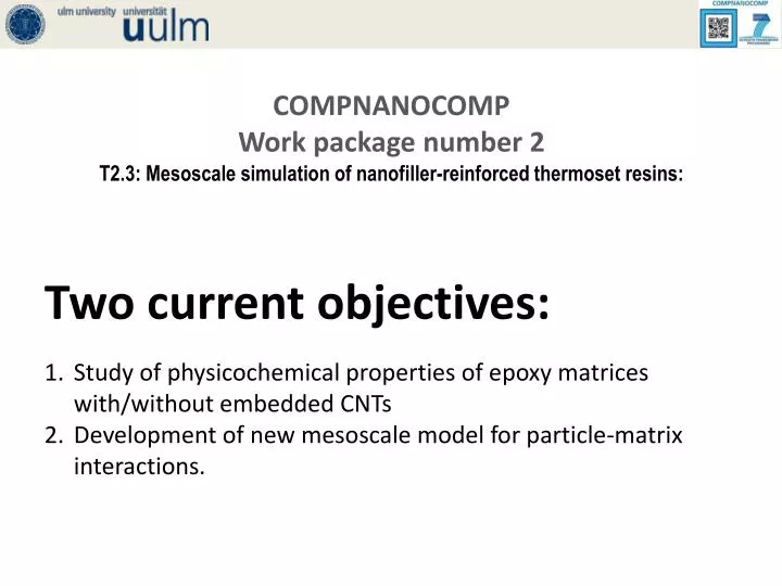
COMPNANOCOMP Work package number 2 T2.3: Mesoscale simulation of nanofiller -reinforced thermoset resins:. Two current objectives : Study of physicochemical properties of epoxy matrices with/without embedded CNTs Development of new mesoscale model for particle-matrix interactions.

E N D
COMPNANOCOMP Work package number 2 T2.3: Mesoscale simulation of nanofiller-reinforced thermoset resins: Two current objectives: Study of physicochemical properties of epoxy matrices with/without embedded CNTs Development of new mesoscale model for particle-matrix interactions.
Part 1: Atomistic simulation of epoxies with/without embedded CNTs Step 1: Using our NG-based method, we convert atomistic species (monomers and CNTs) to coarse-grain representation. Step 2: Using CG monomers, we perform co-polymerization at mesoscale. The reaction proceeds to reach a given degree of conversion. Step 3: After a long equilibration, we convert CG model to atomistic representation.
Step 4: Large-scale fully atomistic simulations of nanotube-reinforced cycloaliphatic epoxy resins are performed with our highly optimized MD code. T < Tg T > Tg
Cycloaliphatic epoxy resins: Properties predicted Density of epoxy matrix as a function of S-DC, at 300 K and 700 K. Volume thermal expansion coefficient of epoxy matrix as a function of S-DC at room temperature (300 K). rcnt≤ r*≈ 1/L3 Reverse density of epoxy matrix as a function of temperature for different conversion ratios. The location of the discontinuity in the slope of the reverse density vs temperature plot indicates the position of the glass transition temperature. rcnt> r*≈ 1/L3 Reverse density as a function of temperature for different CNTs mass fractions. The degree of conversion is 91%. Nanotube length is 5 nm, nanotube diameter is 1.4 nm. The location of the discontinuity in the slope of the reverse density vs temperature plot indicates the position of the glass transition temperatures.
Conclusion: The morphologies and physicochemical properties of filled and unfilled epoxies were studied extensively with fully atomistic simulations. The main parameters of the study are the degree of conversion, temperature, and nanotube content. In particular, our atomistic MD simulations of highly crosslinked epoxies filled with thin carbon nanotubes revealed that these composites exhibit two glass transition temperatures. This behavior is due to the existence of restricted mobility regions (interface regions) in the filled polymers.
Part 2: New mesoscale model for particle-matrix interactions Motivation: The standard CG DPD potentials are purely repulsive and thereby they do not explicitly take into account the adhesive effects between CNTs and polymer matrix. Based on this, it was suggested to modify the model by incorporating the attraction. Two-level description of interactions (implemented in our simulation package) Mesoscale (standard) level "Semi-mesoscale" level
Level 1: Standard (χ-based) parameterization scheme The solubility parameters are used to derive Flory-Huggins interaction values: Here, v0 is the reference volume and δ is the Hildebrand single-component solubility parameter: where Ecoh is the cohesive energy, which is the energy needed to evaporate a system to an ideal gas at constant temperature. Ecoh is calculated from atomistic MD as the average intermolecular energy.
DPD bead The standard DPD model Kuhn segment Lorentz-Berthelot combination rules don't work in mesoscale world εAB Coils are mutually penetrable [Khalatur, Khokhlov. Sov. Phys. Dokl. 1981] σ = characteristic size of bead ε = characteristic energy
In meso- (nacro-) scale world, all interaction parameters can be arbitrary ... εij= εji there is a strong attraction between A and B
Level 2: "Semi-mesoscale" representationExample: PMMA • In "semi-mesoscale" case, what can be DPD beads?
DPD bead ≠ Kuhn segment DPD bead = monomer unit
DPD bead ≠ Kuhn segment DPD bead = monomer unit
DPD bead ≠ Kuhn segment DPD bead = monomer unit do not represent a single covalent bond. non-covalent site-site interaction = the quantity of interest s is simply related to Van der Waals radius of monomer
"Semi-mesoscale" representation of CNT and monomers bead bead bead linker bead CA EM The positions of beads and the topology of inter-bead connections are determined with the Neural-Gas-based algorithm
Site-side interaction between beads: "Semi-mesoscale" model Our aim: effective site-site potentials U(r) U=U(ε,r) with r=|Ri – Rj|; i,j = A,B,C... B B A εAC εBC εBC CNT (C) Main problem: We have to find the functional form of effective potentials U(r)
"Semi-mesoscale" and atomistic models polymer network (atoms or beads) graphite surface (atoms or beads) Atomistic and mesoscale systems
Conversion: 98% Diglycidyl ether of bisphenol A (DGEBA) Amine (DETA)
graphite carbon black mica amorphous silica
Technical details: 1-site and 9-site forces (A) 1-site force (B) 9-site force
Case study: cycloaliphatic epoxy resin (CA and EP monomers) + CNTs Target property: Site-site correlation functions g(r) Atomistic system: Sites = atomic groups (monomers) Mesoscale system: Sites = beads / χ–based potentials CA -graphite CA
Iterative Boltzmann Inversion Initial parameters Start New parameters Optimizer Equilibration No Good agreement? Comparison to atomistic data Yes! Final force-field Simulation and analysis
Iterative Boltzmann Inversion • Perform a target all-atom MD simulation. • For the atomistic system, define pseudoatoms ("beads"). For each pair of bead types, compute the corresponding correlation function (gat). • Estimate the potentials between beads: Ucg(r)/kBT = -ln[gat(r)]. • Perform a mesoscale simulation with the estimated potentials Ucg(r). Compute the correlation functions gcg(r) for the beads. • Update the inter-bead potentials using the following equation: • Go back to step 4 and repeat a DPD simulation. Continue until all Ucg(r) converge.
Case study: Cycloaliphatic epoxy resin CA -graphite repulsion attraction
Deliverable D2.6b Two-level approach to obtain and optimize material-specific coarse-grained potentials for large scale mesoscopic simulation was implemented in our new DPD package.
What should we keep in mind? U(r) is the potential of mean force U(r) is different for different surfaces/nanoperticles U(r) depends on: T, P, density, composition, DC,.... U(r) must be recalculated when any of the parameters is changed U(r) prediction via IBI is very time consuming Strictly speaking, the IBI scheme is wrong for polymer systems...
Truncated Iterative Boltzmann Inversion Truncated correlation function Stress-strain curve attraction
Even in the case of a fantom chain, interacting with an external object, there are strong intrachain correlations influencing the effective site-site potential. These correlations must be explicitly taken into account. To this end, we'll use special intrachain correlation function w(r) and solve numerically the integral pRISM equation.
Integral equation (pRISM) theory The pRISMequation relates the total correlation function, h(r) = g(r)-1, to the intramolecular correlation function, w(r), and the direct correlation function, c(r), via a nonlinear integral equation: the carets ^ denote Fourier transform and is the system density.
Multicomponent system where the asterisks denote convolution integrals, and matrices H, C, W and D consist of the site-site total correlation functions, h(r), the site-site direct correlation functions, c(r), the intramolecular correlation functions, wA(r) and wB(r), and reduced densities A and B, respectively. Here and below, the indexes α and β denote the species A, B, C.... Matrices W and D are given, whereas H and C are calculated.
Solution of pRISM equation The matrix pRISMequation can be solved numerically with an appropriate closure relation. We use the reference Laria-Wu-Chandler closure (R-LWC) where g(r)=h(r)+1 is the pair correlation function and the matrix U is defined as Here, u(sr) is the short-range potential. The superscript "0" refers to correlation functions evaluated at the same density as the system under consideration but without attractive interactions.
The reference correlation functions are calculated by solving the pRISMequation with the standard Percus-Yevick closure
Numerical procedure The correlation functions entering pRISMequation are divided into short-ranged parts and long-ranged parts The corrections to the long-range parts are given by the following matrix equation which is solved iteratively, using an auxiliary iteration function in reciprocal Fourier space: The R-LWC closure relation can now be rewritten as
Picard and Ng iteration schemes The simple iterative method for solving of the pRISMequation can be represented as where denotes the corresponding nonlinear integral operator. Starting with initial guess (0), a sequence of output functions (s+1) is generated. Our procedure (Ng-type scheme) utilizes the input and output auxiliary functions of several previous iteration steps and hence has a much faster converging rate than the usual mixing (Picard) scheme. An "trial" input for the (s+1)th iteration is given by the following linear combination
To find the best possible solution at a current iteration step, we must have the optimal set of the coefficients {ak}. They can be obtained by minimizing of the norm with respect to {ak}. Here, For {ak} we have the following system of linear equations
Having {ak}, the input for the next (s+1)th iteration is defined as For more detail, see the following publications: Khalatur P.G., ZherenkovaL.V., KhokhlovA.R.J. Phys. II (France) 1997, 7, 543. Khalatur P.G., ZherenkovaL.V., KhokhlovA.R.Physica A 1997, 247, 205. KhalaturP.G., ZherenkovaL.V., KhokhlovA.R.Eur. Phys. J. B & D, 1998, 5, 881. Khalatur P.G., KhokhlovA.R.Molec. Phys. 1998, 93, 555. Khalatur P.G., KhokhlovA.R.J. Chem. Phys.. 2000, 112, 4849.
DPD_CHEM = domain-decomposition-based parallel algorithm: Site-site forces
Coupling atomistic and coarse-grained simulations Molecules in atomistic region (Model 1), coarse grain region (Model 2), and transition region (middle). Molecules in the transition region switch in a smooth fashion from one resolution into the other by treating their interaction as partly fully atomistic (FA) and partly coarse grained (CG). This switching is controlled by a scaling function W(R) that goes smoothly from unity to zero (W1) or from zero to unity (W2), depending on the molecule's position R relative to the transition region of thickness d.