Download
1 / 8
80 likes | 263 Views
Two objectives of surrogate fitting. To fit a surrogate we minimize an error measure, called also “loss function.” We also like the surrogate to be simple:. Fewest basis functions Simplest basis functions

E N D
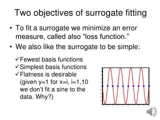
Two objectives of surrogate fitting • To fit a surrogate we minimize an error measure, called also “loss function.” • We also like the surrogate to be simple: • Fewest basis functions • Simplest basis functions • Flatness is desirable (given y=1 for x=i, i=1,10 we don’t fit a sine to the data. Why?)
Support Vector Regression • Combines loss function and flatness as a single objective. • Support vector machines developed by Vapnik and coworkers for optical character recognitions in Russia in the 1960s. • First use for regression in 1997. • Besides regression has become popular as classifier to divide design space into feasible domain (where constraints are satisfied) and infeasible domain (where they are not).
Epsilon-insensitive loss function • Support vector regression can use any loss function, but the one most often associated with it is epsilon-insensitive. • It is less sensitive to one bad data point. Figures from Gunn’s Support Vector Machines for Classification and Regression
Flatness measure • Take a surrogate , where the are shape functions and are coefficients. • A possible flatness measure is , where is a measure of the curvature associated with the ith shape function. • For example, the constant term should have a zero .
SVR optimization problem • The coefficients of the surrogate are found by solving the following optimization problem • This is a challenging optimization problem because the loss function is not a smooth function of the coefficient. • A well behaved constrained formulation is given in the notes.
Example • Four strain-stress measurements are given: ε=[1,2,3,4] milistrainsσ=[10,22,33,35] ksi. • Fit an SVR surrogate to the data of the form , assuming that the stress is accurate up to 2 ksi. • Assign zero flatness to the linear coefficient and =1, or =100 to the quadratic coefficient. • You may use Matlab’sfminsearch for the optimization, since it is not a gradient based method.
Solution • Figure compares the two fits • For =1, =12.9, the loss function dominates. • Errors at data points are: -2.00 -0.17 2.50 -2.00 • For =100, 0.025; flatness is important • Errors at data points are: -0.025 2.00 3.075 -4.80 • Matlab commands given in notes.
Problems • Fit a linear polynomial and a quadratic polynomial to the data of the example using linear regression (e.g. Matlab’spolyfit or regress). Compare to the SVR fits and comments. • Assume that the exact stress-strain law is . Generate data at 11 equispaced points in [1,4] contaminated by normal random noise of zero mean and standard deviation of 1. Perform the SVR fits for the two values of the flatness and the two linear regression fits. Compare and comment.