Download
1 / 28
290 likes | 807 Views
Vectors. Objectives. Understand the notion of vectors Distinguish between points and vectors Introduce the concept of homogenous coordinate systems Get familiar with some applications of vectors in computer graphics. Vectors. Vectors provide easy ways of solving some tough problems.

E N D
Objectives • Understand the notion of vectors • Distinguish between points and vectors • Introduce the concept of homogenous coordinate systems • Get familiar with some applications of vectors in computer graphics
Vectors • Vectors provide easy ways of solving some tough problems. • Physical definition: a vector is a quantity with two attributes • Direction • Magnitude • Examples include • Force • Displacement • Velocity • Acceleration • Directed line segments • Most important example for graphics • Can map to other types v
Vector Operations • Every vector has an inverse • Same magnitude but points in opposite direction • Every vector can be multiplied by a scalar • There is a zero vector • Zero magnitude, undefined orientation • The sum of any two vectors is a vector • Use head-to-tail axiom
Vector Operations (2) • Subtracting c from a is equivalent to adding a and (-c), where –c = (-1)c.
Vector representation • We represent an n-dimensional vector by an n-tuple of its components, e.g. v = (vx, vy, vz). • We will usually use 2, 3, or 4 dimensional vectors: e.g., v=(3, -2), u=(3,2,2), t=(3,2,4,1). • A vector v = (33, 142.7, 89.1) is a row vector. • A vector v = (33, 142.7, 89.1)T is a column vector. • It is the same as
Vectors Lack Position • These vectors are identical • Same direction and magnitude • Vectors spaces insufficient for geometry • Need points
Points vs vectors • Location in space • Operations allowed between points and vectors • Subtracting two points yields a vector • Adding a point to a vector gives a point A vector v between points P = (1, 3) and Q = (4, 1), has the components (3, -2), calculated by subtracting the coordinates individually (Q – P).
Linear Vector Spaces • Mathematical system for manipulating vectors • Operations • Scalar-vector multiplication u = av • E.g. sv = (svx, svy, svz) • Vector-vector addition: w = u + v • E.g v1 ± v2 = (v1x ± v2x, v1y ± v2y, v1z ± v2z) • Expressions such as v=u+2w-3r Make sense in a vector space • A linear combination of the m vectors v1, v2, …, vm is any vector of the form a1v1 + a2v2 + … + amvm. • Example: 2(3, 4,-1) + 6(-1, 0, 2) forms the vector (0, 8, 10).
Linear Combinations of Vectors • The linear combination becomes an affine combination if a1 + a2 + … + am = 1. • Example: 3a + 2 b - 4 c is an affine combination of a, b, and c, but 3 a + b - 4 c is not. • (1-t) a + (t) b is an affine combination of a and b. • The affine combination becomes a convex combination if ai ≥ 0 for 1 ≤ i ≤ m. • Example: .3a+.7b is a convex combination of a and b, but 1.8a -.8b is not.
The Set of All Convex Combinations of 2 or 3 Vectors • v = (1 – a)v1 + av2, as a varies from 0 to 1, gives the set of all convex combinations of v1 and v2. An example is shown below.
Vector Magnitude and Unit Vectors • The magnitude (length, size) of n-vector w is written |w|. • Example: the magnitude of w = (4, -2) is and that of w = (1, -3, 2) is . • A unit vector has magnitude |v| = 1. • The unit vector pointing in the same direction as vector a is (|a| ≠0): • Converting a to is called normalizing vector a.
Vector Dot Product • The dot product of n-vectors v and w is v∙w = v1w1 + v2w2 + … + vnwn • The dot product is commutative: v∙w = w∙v • The dot product is distributive: (a ± b)∙c = a∙c ± b∙c • The dot product is associative over multiplication by a scalar: (ta)∙b = t(a∙b) • The dot product of a vector with itself is its magnitude squared: b∙b = |b|2
Angle Between two Vectors • b = (|b| cos φb, |b| sin φb), and c = (|c| cos φc, |c| sin φc) • b∙c = |b||c| cos φc cos φb + |b||c| sin φb sin φc = |b||c| cos (φc- φb) = |b||c| cos θ, where θ = φc- φb is the smaller angle between b and c: • The sign of dot product:
Perpendicular Vector • A vector b is perpendicular to a vector a iff a.b = 0. • In 2D, If vector a = (ax, ay), then the vector perpendicular to a • In the counterclockwise sense: a┴ = (-ay, ax) • In the clockwise sense it is -a┴. • In 3D, any vector in the plane perpendicular to a is a perpendicular to a.
Properties of ┴ • (a ± b)┴ = a┴ ± b┴; • (sa)┴ = s(a┴); • (a┴)┴ = -a • a┴ ∙ b = -b┴ ∙ a = -aybx + axby; • a┴ ∙ a = a ∙ a┴ = 0; • |a┴| = |a|;
Orthogonal Projections and Distance from a Line • We are given two points A and C and a vector v. The following questions arise: • How far is C from the line L that passes through A in direction v? • If we drop a perpendicular onto L from C, where does it hit L? • How do we decompose a vector c = C – A into a part along L and a part perpendicular to L?
Illustration of Questions • We may write c = Kv + Mv┴. If we take the dot product of each side with v, we obtain c∙v = Kv∙v + Mv┴∙v = K|v|2 (why?), or K = c∙v/|v|2. • Likewise, taking the dot product withv┴ gives M = c∙v┴/|v|2. (Why not |v┴|2 ?) • Answers to the original questions: Mv┴, Kv, and both.
Reflections • Can happen with lights or objects • When light reflects from a mirror, the angle of reflection must equal the angle of incidence: θ1 = θ2. • Vectors and projections allow us to compute the new direction r, in either two-dimensions or three dimensions.
Example on Reflection • The illustration shows that • e = a – m • r = e – m = a – 2m • m = [(a∙n)/|n|2]n = Thus, r =
Vector Cross Product (3D Vectors Only) • axb=(aybz – azby)i + (azbx – axbz)j + (axby – aybx)k. • The determinant below also gives the result:
Cross-Product Properties • i x j = k; j x k = i; k x i = j • a x b = - b x a; a x (b ± c) = a x b ± a x c; (sa) x b = s(a x b) • a x (b x c) ≠ (a x b) x c – for example, a = (ax, ay, 0), b = (bx, by, 0), c = (0, 0, cz) • c = a x b is perpendicular to a and to b. The direction of c is given by a right/left hand rule in a right/left-handed coordinate system.
Properties (2) • a ∙ (a x b) = 0 • a x b = |a||b| sin θ, where θ is the smaller angle between a and b. • a x b is also the area of the parallelogram formed by a and b. • a x b = 0 if a and b are linearly dependent.
Application: Finding the Normal to a Plane • Given any 3 non-collinear points A, B, and C in a plane, we can find a normal to the plane: • a = B – A, b = C – A, n = a x b. The normal on the other side of the plane is –n.
Point + Vector • Suppose we add a point A and a vector that has been scaled by a factor t: the result is a point, P = A + tv. • Now suppose v = B – A, the difference of 2 points: P = tB + (1-t)A, an affine combination of points. • P is a point on the line that passes through A and B (i.e. the line that passes through A and parallel to the vector v)
Linear Interpolation • P = (1-t)A + tB is a linear interpolation (lerp) of two points. • Px (t) provides an x value that is fraction t of the way between Ax and Bx. (Likewise Py(t), Pz(t)). float lerp (float a, float b, float t){ return a + (b – a) * t; } • Used for tweening and in animation • In films, artists draw only the key frames of an animation sequence (usually the first and last). • Tweening is used to generate the in-between frames.
Practice session: Use the ideas covered in this lecture to compute the intersection of a line and a plane.