General Competitive Equilibrium

1. General Competitive Equilibrium Chapter 11

2. Introduction • In general, changes in one market will affect demand and supply in other markets • General-equilibrium analysis • Study of how demand and supply conditions interact in a number of markets and determine prices of many commodities • Economy is viewed as a closed and interrelated system • Where interactions of all markets determine equilibrium market prices and quantities • Disturbance in one market generates ripples that spread through many other markets • A (general) equilibrium model of all markets will result in necessary conditions for economic efficiency • Achieved by agents (households and firms) trading commodities • Agents will engage in trade until all gains from trade are exhausted

3. Introduction • This chapter no longer restricts supply of commodities to sum of individual agents’ initial endowments • Allows firms to employ these endowments as inputs into production and produce some outputs that will increase supply of those commodities • With introduction of production, conditions yielding production efficiency are now required for economic efficiency • Allocation conditions for production efficiency • Allocation Condition 1 (opportunity cost condition) • Obtained by deriving production possibilities frontier • Where production must occur for efficiency • Allocation Condition 2, (marginal product condition) • For efficiency inputs should be allocated so that marginal products in production of a particular commodity are equal • Allocation Condition 3 (comparative advantage condition) • For efficient production a firm with comparative advantage in producing a commodity should produce that commodity

4. Introduction • Conditions for overall economic efficiency • Must link producers’ efficient production decisions with consumers’ preferences • An economy may be production efficient • But if it is not producing commodities consumers desire, it is inefficient • Aim in this chapter • Demonstrate how a perfectly competitive market will result in an efficient allocation of a society’s resources • Based on link between economic efficiency and competitive markets • Applied economists are able to investigate effects that various policies have • On directly affected market • On related markets • With this general analysis of markets throughout economy, economists can determine complete impact of policies on an economy • Failure to consider all effects across all markets may result in erroneous analysis • Wrong prescriptions for curing market imperfections

5. Efficiency in Production • Can extend concept of Pareto efficiency and Edgeworth box to production efficiency • Efficiency in production deals with allocation of resources (inputs) within a specific firm • As well as how resources and outputs should be allocated among firms • Generally, an allocation of resources is production efficient • When no reallocation of resources will yield an increase in one commodity without a sacrifice in output from other commodities • Necessary conditions for such an efficiency are stated in three allocation conditions • Opportunity cost condition • Marginal product condition • Comparative advantage condition

6. Allocation Condition 1 (Opportunity Cost Condition) • For production efficiency no more of one commodity can be produced without having to cut back on production of other commodities • Requires that MRTS for each output be equal • Consider optimal choice of inputs for a single firm producing two outputs (fish, F, and bread, B) • With two inputs (capital, K, and labor, L) • Assuming limited resources and holding total quantities of K and L fixed • Problem is how to efficiently allocate these fixed resources to production of F and B • Firm will operate efficiently if it is not possible to reallocate its inputs in such a way that output of F can be increased without cutting back on B

7. Allocation Condition 1 (Opportunity Cost Condition) • Firm with fixed resources has allocated its resources efficiently if it has them fully employed and • MRTS between inputs is same for every output firm produces • Suppose firm has 100 units of L and 100 units of K • Uses half of each input to produce fish and bread • If firm employs 50 units of K and 50 units of L to produce fish and MRTSF (K for L) = 2 • Same amount of fish could be produced by employing 48 units of K and 51 units of L (See Table 11.1)

8. Table 11.1 Allocation Condition 1 (Opportunity Cost Condition)

9. Allocation Condition 1 (Opportunity Cost Condition) • Represented graphically in Figure 11.1 • Edgeworth box is analogous to box representing pure-exchange model in Chapter 6 • Compares various output levels for fish and bread with isoquants • Illustrates that every point inside box represents a feasible allocation • Origin 0F • Allocation where no resources are allocated to fish production (0, 0) and all resources are devoted to bread production (100, 100) is a feasible allocation represented by the • Output of bread is maximized and no fish is produced • At 0B, allocation is (0, 0) toward production of bread and (100, 100) for fish • For a movement toward 0F, more of K and L are being allocated toward bread production and less toward fish • Every feasible combination of K and L in production of fish and bread is represented inside Edgeworth box • Points outside the box are not feasible

10. Figure 11.1 Allocation Condition 1

11. Allocation Condition 1 (Opportunity Cost Condition) • Size of box is determined by amount of fixed resources, K and L • An increase in amount of resources will enlarge box • A change in technology for combining resources to produce outputs may also expand output potential but not size of box • Production-efficient allocations are characterized by efficiency locus in Figure 11.1 • Called production contract curve • Represents set of efficient allocations • At every point on production contract curve MRTSF= MRTSB

12. Allocation Condition 1 (Opportunity Cost Condition) • In Figure 11.1, point C is not Pareto efficient • Possible to reallocate inputs in such a manner that one product can be increased without reducing other product • For example, moving along bread isoquant curve toward point P3 • Bread production remains unchanged but fish production increases • Mathematically, efficiency condition MRTSF =MRTSB is determined by maximizing one output while holding other output constant

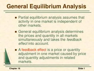
13. Production Possibilities Frontier • In U.S., over 40% of all scientists, engineers, and technical professionals work in military defense sector • Allocation of talent and intellectual resources could be used for other production possibilities • Based on efficiency locus in Figure 11.1, these alternative production possibilities for commodities (guns and butter or fish and bread) can be illustrated by production possibilities frontier (See Figure 11.2) • A mapping of efficient output levels, F and B, for each point on production contract curve • Corresponding output levels for fish (F1, F2, F3, and F4) and bread (B1, B2, B3, and B4) are plotted on horizontal and vertical axes in Figure 11.2

14. Figure 11.2 Production possibilities frontier

15. Production Possibilities Frontier • Points on production possibilities frontier correspond to tangency of isoquants along production contract curve in Figure 11.1 • Output combinations (F1,B1), (F2,B2), (F3,B3 ), and (F4,B4) associated with (P1, P2, P3, and P4) are same for both figures • Every point inside production possibilities frontier is a feasible allocation • Corresponding to points inside Edgeworth box in Figure 11.1 • Boundary of production possibilities frontier represents efficiency locus (production contract curve) in Figure 11.1 • For given amounts of K and L, production possibilities frontier indicates combinations of F and B that can be produced • An increase in amount of K and L or an improvement in technology will result in production possibilities frontier shifting outward

16. Marginal Rate of Product Transformation • Slope of production possibilities frontier measures how output F can be substituted for output B • When total level of inputs (resources) is held constant • Negative of this slope is called marginal rate of product transformation (MRPT) • MRPT (B for F) = -slope of production possibilities frontier • MRPT (B for F) = -dB/dF|holding input constant • Slope of production possibilities frontier is negative • Given production efficiency, an increase in one output will require a sacrifice in other output • Taking negative of this negative slope yields a positive MRPT • MRPT measures how much one commodity is sacrificed to produce an additional amount of another commodity • At point P1 in Figure 11.2, MRPT is a relatively small number • Sacrifice in B for an additional unit of F is small • At point P4 MRPT is a relatively large number • Sacrifice in B for an additional unit of F is large • Increase in MRPT as F increases is due to concave nature of production possibility frontier

17. Concave Production Possibilities Frontier • Concave shape of production possibilities frontier is characteristic of most production situations • Based on technical relationship exhibited by two outputs • Can represent total cost of producing F and B by total cost function TC(F, B) • Given fixed level of input supply, cost is constant along production possibilities frontier • Total differential of this cost function is • dTC = (∂TC/∂F)dF + (∂TC/∂B)dB = 0 • dTC is equal to zero because cost is constant along production possibilities frontier • Rearranging terms results in • MRPT(B for F) = -dB/dF|dTC=0 = (∂TC/∂F)/( (∂TC/∂B) = MCF/MCB • In general MRPT(q2 for q1) = MC1/MC2

18. Concave Production Possibilities Frontier • Can compare relationship of MRPT equaling ratio of marginal costs to allocation of inputs for production of F and B • Recall that for one variable input—say, labor • MCF = w/MPL|F • MCB = w/MPL|B • MPL|F (MPL|B) is marginal product of labor in production of fish (bread) • Assume it takes 1 unit of L to produce 2 units of F, MPF = 2; if wage rate is 1 • MCF = ½ • For a concave production possibilities frontier (as illustrated in Figure 11.2) • Ratio of MCF to MCB increases as output of F increases and B decreases • In short run, this is result of Law of Diminishing Marginal Returns • An increase in F results in an increase in its SMC • Decrease in B results in a decrease in its SMC • In long run, a concave production possibilities frontier will also result if decreasing returns to scale exists for both outputs • LMC curves have a positive slope

19. Concave Production Possibilities Frontier • Specialized inputs exist when some inputs are relatively more suited for production of a particular output • Have a comparative advantage in production of one output versus another • In Figure 11.2, concave nature of production possibilities curve implies that increases in F production requires taking inputs out of B production • Where they are more suitable • Allocating them to F production • Where they are progressively less suitable • As production of F increases and that of B declines • Marginal cost for F production increases and marginal cost for B production decreases • Yields a relatively larger MRPT • Specialized inputs assume heterogeneous inputs • Even if inputs are homogeneous, production possibilities frontier will be concave if production of F and B use inputs in different proportions • Different input intensities are represented by nonlinear production contract curves

20. Concave Production Possibilities Frontier • In Figure 11.3 production contract curve is bowed above main diagonal • Indicates that production of F is relatively more capital intensive than that of B • If curve were bowed below main diagonal • B would be relatively more capital intensive • Production possibilities frontier will be concave if production contract curve is not linear through origin of both F and B • Consider Figure 11.3, where F is using a high proportion of capital relative to B • Weighted average of points P1 and P2 is represented by linear cord connecting points • Points on this cord result in a lower level of output for both F and B • Compared to points on production contract curve • In terms of corresponding production possibilities frontier, Figure 11.4 • Cord lies in interior of mapping that establishes concave nature of frontier

21. Figure 11.3 Production contract curve with weighted average of outputs

22. Figure 11.4 Production possibilities frontier with differing factor intensities

23. Opportunity Costs • Production possibilities frontier illustrates a fundamental condition in economic theory • Assuming resources are fully employed in most efficient way • Any increase in production of one commodity will require shifting of resources out of other commodity and vice versa • Opportunity cost of producing more of the one commodity • MRPT measures degree of opportunity cost • A relatively large MRPT = -dB/dF|dTC=0 • Illustrates a large opportunity cost of increasing F • Concave production possibilities frontier is associated with increasing opportunity cost • The more concave the frontier • The greater the increase in opportunity cost as one commodity is sacrificed for production of another • Constant MRPT implies a linear production possibilities frontier and constant opportunity cost • Theoretically, if factor intensities are the same and production functions exhibit increasing returns to scale • Production possibilities frontier will be convex • Represents decreasing opportunity cost as one commodity is substituted for another

24. Economies of Scope • Increasing opportunity cost results in lowest opportunity cost for increasing fish corresponding to point A • At point A, production of fish is zero • Lowest opportunity cost for producing bread is at point B • Production of bread is zero • Low levels of opportunity cost result from joint production of fish and bread • In general, a firm incurs production advantages when it produces two or more products • Can use inputs and technologies common to producing a set of products • May be advantages in joint use of inputs, marketing programs, or administration

25. Economies of Scope • Unless there are some constraints firms will almost always produce more than one product • Technologies resulting in joint production advantages are called economies of scope or increasing returns to scope • Exist when one firm jointly producing a set of products results in a higher level of output than a set of separate firms each uniquely producing one of the products • Results in concave production possibilities curves • Without these production advantages associated with joint production • Joint production would generate same output as the two specialized firms • Production possibilities frontier would be linear • Representing constant opportunity cost or constant returns to scope

26. Diseconomies of Scope • Decreasing opportunity cost associated with convex production possibilities frontiers characterize diseconomies of scope (decreasing returns to scope) • Illustrated in Figure 11.5 • Opportunity cost of specialization is lower than cost of joint production • Production possibilities frontier is below cord connecting points A and B • At point A in Figure 11.5, increasing fish production • Results in MRPT on convex production possibilities frontier being greater than MRPT on cord between points A and B • Opportunity cost of producing fish and bread jointly is greater than opportunity cost of specialized production • There is no direct relationship between economies to scale and economies of scope • Economies of scale is concerned with output effect of expanding production through increasing all inputs • Economies of scope is concerned with output effect of expanding production through increasing number of different products produced • Both are related to increasing output • But differ in how output is increased • Returns to scale increases output through input usage • Returns to scope increases output through product diversification

27. Figure 11.5 Decreasing returns to scope, decreasing opportunity cost, and …

28. Allocation Condition 2 (Marginal Product Condition) • If production is to be efficient, resources should be allocated to point where marginal product of any resource in production of a particular commodity is the same • No matter which firm produces the commodity • For example, consider two firms (1 and 2) producing the same commodity, Q • An objective of society is to determine efficient allocation of K and L between the two firms that will maximize output, Q

29. Allocation Condition 2 (Marginal Product Condition) • Incorporating constraints into objective function yields

30. Allocation Condition 2 (Marginal Product Condition) • In general, for N firms, F.O.C.s result in Allocation Condition 2 (marginal product condition) • MPK|firm 1 = MPK|firm 2 = … = MPK|firm n • MPL|firm 1 = MPL|firm 2 = … = MPL|firm n • For labor input with two firms this allocation condition is illustrated in Figure 11.6 • If MPL|firm 1 > MPL|firm 2 • Can increase combined output for both firms by reallocating labor inputs • Area under a marginal product curve is total amount of output produced • Shaded areas represent change in output • Shaded area associated with firm 1 is larger than shaded area for firm 2 • Net gain in output represents increase in output by reallocating input • Can continue to increase output by shifting input allocation until level of the input used by each firm results in equivalent marginal products

31. Figure 11.6 Allocation Condition 2

32. Allocation Condition 2 (Marginal Product Condition) • Alternative illustration of Allocation Condition 2 for production functions of two firms producing the same commodity, Q, with one variable input, L • Shown in Figure 11.7 • Can increase total output of Q with given amount of labor, L • By reallocating labor between two firms • Taking labor away from less productive firm 1 • Allocate it to relatively more productive firm, firm 2 • Will enlarge box vertically • Output will continue to increase for given level of labor • Until production functions are tangent • At this tangency, marginal products for these two firms will be equal • Results in an efficient allocation of labor for production of Q • Indicated in Figure 11.8 • Q* in Figure 11.8 is greater than Q'in Figure 11.7

33. Figure 11.7 Inefficient allocation of labor between two firms

34. Figure 11.8 Allocation Condition 2 with an Edgeworth box

35. Allocation Condition 3 (Comparative Advantage Condition) • If two or more firms produce same outputs • They must operate at points on their respective production possibility frontiers • At which marginal rates of product transformation are equal • Figure 11.9 illustrates this Pareto-efficient condition • At point A MRPT for firm 1 is greater than MRPT for firm 2 • By reallocating production of outputs between the two firms • Can reduce total amount of resources employed for producing given amount of fish and bread • Only where MRPTs for two firms are equal is it impossible to reallocate production in such a way as to reduce resource requirements for given level of production

36. Figure 11.9 Allocation Condition 3

37. Comparative Advantage • Related to Allocation Condition 3 is theory of comparative advantage in international trade • First developed by David Ricardo • A country has a comparative advantage in commodities that it is relatively more efficient in producing • Efficiency is measured in the sacrifice of other commodities for production of an additional unit of a commodity • Comparative advantage is in contrast to absolute advantage • A country’s cost in terms of input usage is used as measure of advantage • Countries will specialize in producing products for which they have a comparative advantage until their MRPTs are equilibrated • Will then trade with other countries to satisfy consumer demand

38. Comparative Advantage • As countries specialize in production of commodity for which they have a comparative advantage • Gains from improved efficiency are realized • Ability to either produce more of both commodities or • Maintain their current production levels and allocate excess resources to other activities • Total world production will increase • Improved efficiency through comparative advantage and trade is basis for supporting idea of reducing trade barriers

39. Economic Efficiency • If all three allocation conditions for production and equality of MRS exchange condition hold • Provides for a Pareto-efficient production and exchange of commodities • However, they are not sufficient for achieving economic efficiency • Also require output efficiency • What firms produce is what households want • For example, an economy that concentrates on efficient production of military commodities at expense of household items during relative peace is inefficient • Requires that MRS = MRPT • MRS measures how much a household is willing to substitute one commodity for another, holding utility constant • MRPT measures opportunity cost (sacrifice of another commodity) of producing one more unit of a commodity • If MRS > MRPT, household’s willingness to substitute one commodity for another is greater than opportunity cost • Efficiency can be improved by a reallocation of resources until a household’s willingness-to-pay is equal to cost of producing any additional unit of a commodity

40. One-household Or Homogeneous Preferences Economy • Concept of equating MRS to MRPT is illustrated in Figure 11.10 for case of a one-household economy • Or case where all households have same utility function • Assume this household (or set of households acting as one) produces and consumes two commodities with a given level of inputs • Household’s preferences for two commodities are represented by indifference curves superimposed on household’s production possibilities frontier • Household attempts to maximize utility subject to production possibilities constraint

41. Figure 11.10 Economic efficiency for a one-household economy

42. One-household or Homogeneous Preferences Economy • At commodity bundle A, MRS(x2 for x1) > MRPT(x2 for x1) • The one household can increase its utility by moving down along production possibilities frontier from A to B • At bundle B, household is maximizing its utility for this production possibilities frontier • Corresponds to where MRS(x2 for x1) = MRPT(x2 for x1) • Economically efficient commodity bundle (Pareto-efficient allocation) for the economy • Point where society maximizes social welfare, local bliss • Because there is only one household in this economy • Bundle B is only point on production possibilities frontier where there is no other commodity bundle preferred to it • For example, bundle A is Pareto efficient in terms of production • But there are commodity bundles, such as C, within production possibilities frontier that are preferred to A • Bundle C is inefficient in terms of production • Because it is in interior of production possibilities frontier

43. Pareto Efficiency With More Than One Type Of Household Preferences • In Chapter 6, general-equilibrium condition for a pure-exchange economy with n households equated MRS across all households • By combining this pure-exchange condition with equilibrium solution when considering a one-household production economy, MRS = MRPT • Get necessary conditions for a Pareto-efficient allocation • When there are more than one type of household preferences, a Pareto-efficient allocation requires that • MRS1 = MRS2 = … = MRSn = MRPT • If all n households have the same preferences for the commodities • Their MRSs will be the same and a Pareto-efficient allocation for more than one type of household preferences reduces to one-household production economy solution • MRS =MRPT

44. Two-Household Economy with Heterogeneous Preferences • Assuming Friday and Robinson have different preferences, we must examine economic efficiency associated with more than one type of household preferences • Pareto-efficient allocation is where MRS for Robinson equals MRS for Friday and both are equal to MRPT • Illustrated in Figure 11.11 • Production-efficient commodities, Q1* and Q2*, from production possibilities frontier, forms an Edgeworth box • Robinson’s indifference map originates from production possibilities frontier point of origin, 0R • Friday’s indifference map is rotated 180with its origin placed on production possibilities frontier associated with Q1* and Q2* • At point where Robinson’s and Friday’s MRSs are equal and MRPT is also equal to their MRSs • Pareto-efficient allocation exists

45. Figure 11.11 Economic efficiency for a two-household economy

46. Figure 11.12 Economic efficiency for alternative utility levels

47. Two-Household Economy with Heterogeneous Preferences • Mathematically, we derive the condition MRSR = MRSF = MRPT by maximizing Robinson’s utility subject to • Friday’s utility • Production possibilities constraint • And condition that what is being produced (supply) must equal demand • If all commodities are desirable, then an efficient allocation would have no excess demand • Supply would equal demand • This Pareto-efficiency allocation, illustrated in Figure 11.11, is based on a given level of utility for Friday • Changing this level of utility for Friday will result in alternative combinations of Q1 and Q2 produced and allocated between Robinson and Friday • Maximizing Robinson’s utility results in Pareto-efficient allocation • Illustrated in Figure 11.12

48. Two-Household Economy with Heterogeneous Preferences • In general, considering all possible Pareto-efficient allocations, MRSR = MRSF = MRPT • By varying Friday’s utility from consuming zero units of Q1 and Q2 to Friday consuming all of Q1 and Q2 • Obtain a collection of all economically efficient utility levels (contract curve) for both Robinson and Friday • Initial endowment of resources held by Robinson and Friday will determine which of these economically efficient allocations are feasible • For example, if Friday initially has a relatively large share of resources • An economically efficient allocation resulting in Robinson consuming most of the commodities would not be feasible • Competitive-price system will yield an economically efficient allocation • However, initial allocation of endowments or access to these endowments (equal opportunity) has social-welfare implications • Redistribution of initial endowments may enhance social welfare and thus be socially desirable

49. General Equilibrium in a Competitive Economy • A perfectly competitive economy assumes agents (households and producers) take all prices as given • No agent has control over some of the markets and, thus, no agent can influence market prices • In this economy, a general competitive equilibrium is a set of prices for both inputs and outputs • Where quantity demanded equals quantity supplied in all input and output markets, simultaneously • At this set of prices, households maximize utility subject to their initial endowments and firms maximize profit

50. Efficiency In Production • Can establish a relationship between this competitive-equilibrium set of prices and efficiency in production by examining three allocation conditions • Perfectly competitive pricing provides necessary conditions for these allocation conditions to hold • Recall Allocation Condition 1 • MRTS1 =MRTS2 = … =MRTSk =w*/v*, for all k commodities • Where the two inputs are labor and capital with a wage rate of w and a rental rate of v • Given perfect competition in input markets, firms producing these k commodities will equate their MRTS(K for L) to common input price ratio, w*/v*, which results in Allocation Condition 1 • Thus, in a decentralized tâtonnement process, without any market intervention, firms will adopt least-cost combination of inputs for a given level of output