Download
1 / 40
400 likes | 621 Views
Chapter 6 Classification and Prediction (1). Outline. Classification and Prediction Decision Tree Naïve Bayes Classifier Support Vector Machines (SVM) K-nearest Neighbors Other Classification methods Accuracy and Error Measures Ensemble Methods Applications Summary.

E N D
Chapter 6Classification and Prediction (1) CISC 4631
Outline • Classification and Prediction • Decision Tree • Naïve Bayes Classifier • Support Vector Machines (SVM) • K-nearest Neighbors • Other Classification methods • Accuracy and Error Measures • Ensemble Methods • Applications • Summary CISC 4631
Supervised vs. Unsupervised Learning Supervised learning (classification) Supervision: The training data (observations, measurements, etc.) are accompanied by labels indicating the class of the observations New data is classified based on the training set Unsupervised learning (clustering) The class labels of training data is unknown Given a set of measurements, observations, etc. with the aim of establishing the existence of classes or clusters in the data CISC 4631
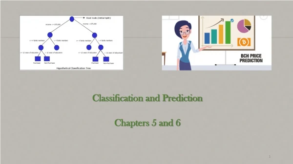
Classification classifies data (constructs a model) based on the training set and the values (class labels) in a classifying attribute and uses it in classifying new data predicts categorical class labels Prediction models continuous-valued functions, i.e., predicts unknown or missing values Regression analysis: a statistical method Predict how much a given customer will spend during a sale. Classification vs. Prediction CISC 4631 4
Typical applications Credit/loan approval: Medical diagnosis: if a tumor is cancerous or benign Fraud detection: if a transaction is fraudulent Web page categorization: which category it is Application of Classification CISC 4631
Classification—A Two-Step Process Model construction: describing a set of pre-determined classes Each tuple/sample is assumed to belong to a predefined class, as determined by the class label attribute The set of tuples used for model construction is training set The model is represented as classification rules, decision trees, or mathematical formulae CISC 4631
Classification—A Two-Step Process • Model usage: for classifying future or unknown objects • Estimate accuracy of the model • The known label of test sample is compared with the classified result from the model • Accuracy rate is the percentage of test set samples that are correctly classified by the model • Test set is independent of training set, otherwise over-fitting will occur • If the accuracy is acceptable, use the model to classify data tuples whose class labels are not known. CISC 4631
Process (1): Model Construction Classification Algorithms Training Data Classifier (Model) IF rank = ‘professor’ OR years > 6 THEN tenured = ‘yes’ CISC 4631
Process (2): Using the Model in Prediction Classifier Testing Data Unseen Data (Jeff, Professor, 8) Tenured? CISC 4631
Issues: Data Preparation Data cleaning Preprocess data in order to reduce noise and handle missing values Relevance analysis (feature selection) Remove the irrelevant or redundant attributes Data transformation Generalize and/or normalize data CISC 4631
Issues: Evaluating Classification Methods Accuracy classifier accuracy: predicting class label Speed time to construct the model (training time) time to use the model (classification/prediction time) Robustness: handling noise and missing values Scalability: efficiency in disk-resident databases Interpretability understanding and insight provided by the model Other measures, e.g., goodness of rules, such as decision tree size or compactness of classification rules CISC 4631
Outline • Classification and Prediction • Decision Tree • Naïve Bayes Classifier • Support Vector Machines (SVM) • K-nearest Neighbors • Other Classification methods • Accuracy and Error Measures • Feature Selection Methods • Ensemble Methods • Applications • Summary CISC 4631
Age > 30 Yes No Student? Credit > 600 No Yes Yes No Yes No No Yes Decision Tree • A flowchart-like tree structure. • Internal (non-leaf) node denotes a test on an attribute (feature) • Branch represents an outcome of the test • Leaf node holds a class label. CISC 4631
Output: A Decision Tree for “buys_computer” age? <=30 overcast >40 31..40 student? credit rating? yes excellent fair no yes no yes no yes CISC 4631
Visualization of a Decision Tree in SGI/MineSet 3.0 CISC 4631 May 24, 2014 Data Mining: Concepts and Techniques 16
Algorithm for Decision Tree Induction A greedy algorithm: top-down recursive divide-and-conquer manner. At start, all the training examples are at the topmost node. Examples are partitioned recursively based on selected attributes Test attributes are selected on the basis of a heuristic or statistical measure (e.g., information gain) CISC 4631
Golf Data CISC 4631
Steps of Decision Tree Induction Algorithm • Starts with three parameters: • D, data partition, the set of training tuples and their class labels. • Example: Golf_data: 14 tuples ( 5 yes, 9 no) • Attribute_list, the set of candidate attributes. • Example: {outlook, temp, humidity, windy} • Attribute_selection_method, the procedure to determine the splitting critierion that best partitions the data tuples into individual classes. CISC 4631
Steps of Decision Tree Induction Algorithm • Step 1 (Top-down) • The tree starts with a single node N, representing the training tuples in D. • Step 2 • IF the tuples in D are all of the same class, then node N is a leaf and is labeled with the class label. • ELSEAttribute_selection_method determine the splitting criterion to perform Partitioning of D into Djs. (Divide & Conquer) • Step 3 (Recursive) • Form a decision tree for the tuples at each partition Dj. CISC 4631
Splitting Criterion • Determines the best way to partition the tuples in D into individual classes – pureness of the partitions Dj at each branch. • Which attribute to test. • Which branches to grow from node N with respect to the outcomes of the test. • What is the split-point or the split-subset. CISC 4631
Color? White Red Blue Green Three Partitioning Scenarios (1) • Attribute is discrete-valued • A branch is created for each known value. • Multiple branches may be generated. CISC 4631
Income <= 42,000 Yes No Three Partitioning Scenarios (2) • Attribute is continuous-valued • Test attribute with the split-point • Binary tree is grown. CISC 4631
Color ∈ {red, green} Yes No Three Partitioning Scenarios (3) • Attribute is discrete-valued and binary tree is needed. • Test attribute with the split-subset • Binary tree is grown. CISC 4631
Algorithm for Decision Tree Induction • Conditions for stopping partitioning • All tuples for a given node belong to the same class • Attribute_list is empty: • majority voting is employed for classifying the leaf • There are no tuples for a given branch Dj • A leaf is created with the majority class in D. CISC 4631
Attribute Selection Method: Information Gain • Select the attribute with the highest information gain • This attribute minimizes the information needed to classify the tuples in the resulting partitions. • Let pi be the probability that an arbitrary tuple in D belongs to class Ci, estimated by |C i, D|/|D| • Expected information (entropy) needed to classify a tuple in D: • Entropy represents the average amount of information needed to identify the class label of a tuple in D. CISC 4631 26
Attribute Selection Method: Information Gain • Attribute A has v distinct values. • A can be used to split D into v partitions, where Dj contains those tuples in D that have outcome aj of A. • If A is selected, we wish each partition Dj is pure. • Information needed (after using A to split D into v partitions) to classify D: • The smaller the information needed, the greater the purity of the partitions. • Information gained by branching on attribute A CISC 4631
Let’s grow one (Golf Data) • Golf Data has two classes • Class 1 (Yes), Class 2 (No) • D: 14 tuples, 5 Yes, 9 No. • p1 = 5/14 & p2 = 9/14 • Info(D) = - 5/14*log2(5/14) – 9/14*log2(9/14) = 0.94 CISC 4631
Attribute Selection • A = outlook has 3 distinct values (sunny, overcast, rain) • Dsunny : 5 tuples, 3 Yes, 2 No, p1= 3/5 & p2 = 2/5 • Info(Dsunny) = -3/5*log2(3/5)-2/5*log2(2/5) = 0.97 • Dovercast : : 4 tuples, 0 Yes, 4 No, p1= 0 & p2 = 1 • Info(Dovercast) = -1*log2(1) = 0 • Drain : 5 tuples, 2 Yes,3 No, p1= 2/5 & p2 = 3/5 • Info(Drain) = -2/5*log2(2/5)-3/5*log2(3/5) = 0.97 • InfoA(D) = 5/14*0.97 + 4/14*0 + 5/14*0.97 = 0.69 CISC 4631
Outlook (5,9) Sun (5) OCa (4) Rain (5) Attribute Selection • Gain(outlook) = 0.94 – 0.69 = 0.25 • Gain(temp) = 0.94 -0.911 = 0.029 • Gain(humidity) = 0.94 -0.704 =0.236 • Gain(windy) =0.94 -0.892 = 0.048 CISC 4631
Outlook sunny rain overcast Humidity Wind YES weak normal strong high NO YES NO YES Decision Tree CISC 4631
Computing Information-Gain for Continuous-Value Attributes Let attribute A be a continuous-valued attribute Must determine the best split point for A Sort the value A in increasing order Typically, the midpoint between each pair of adjacent values is considered as a possible split point (ai+ai+1)/2 is the midpoint between the values of ai and ai+1 Given v values of attribute A, v-1 possible split points. The point with the minimum expected information requirement for A is selected as the split-point for A Split: D1 is the set of tuples in D satisfying A ≤ split-point, and D2 is the set of tuples in D satisfying A > split-point CISC 4631
Gain Ratio for Attribute Selection Information gain measure is biased towards attributes with a large number of values Gain ratio is used to overcome the problem. Split Information: normalization to information gain Represents the potential information generated by splitting D into v partitions. GainRatio(A) = Gain(A)/SplitInfo(A) The attribute with the maximum gain ratio is selected as the splitting attribute CISC 4631
If a data set D contains examples from n classes, gini index, gini(D) is defined as where pj is the probability that an arbitrary tuple in D belongs to class Cj, estimated by |C j, D|/|D| The Gini index considers a binary split for each attribute. All possible subsets of distinct values of discrete-valued Attribute A are checked. A ∈ Sa? All possible split-points of continuous-valued are checked. If a data set D is split on A into two subsets D1 and D2, the gini index gini(D) is defined as Gini Index for Attribute Selection CISC 4631
Gini Index for Attribute Selection • Reduction in Impurity: • The attribute provides the smallest ginisplit(D) (or the largest reduction in impurity) is chosen to split the node (need to enumerate all the possible splitting points for each attribute) CISC 4631
Comparing Attribute Selection Measures These three measures, in general, return good results but Information gain: biased towards multivalued attributes Gain ratio: tends to prefer unbalanced splits in which one partition is much smaller than the others Gini index: biased to multivalued attributes has difficulty when # of classes is large tends to favor tests that result in equal-sized partitions and purity in both partitions CISC 4631
Overfitting and Tree Pruning Overfitting: An induced tree may overfit the training data Too many branches, some may reflect anomalies due to noise or outliers Poor accuracy for unseen samples Two approaches to avoid overfitting Prepruning: Halt tree construction early—do not split a node if this would result in the goodness measure falling below a threshold Difficult to choose an appropriate threshold *Postpruning: Remove branches from a “fully grown” tree—get a sequence of progressively pruned trees Cost complexity algorithm: Use a set of data different from the training data to decide which is the “best pruned tree” CISC 4631
Existing Decision Tree Algorithms • ID3 • Use Information Gain to select attribute to split. • C4.5 • A successor of ID3, uses Gain Ratio to select attribute to split • Handling unavailable values, continuous attribute value range, and pruning the tree. • CART • Use Gini Index to select attribute to split • Cost complexity pruning algorithm with validation set. CISC 4631
Classification Rules from Trees • Easily understandable classification rules • Each leaf is equivalent to a classification rule. • Example: • IF (income > 92.5) AND (Education < 1.5) AND (Family ≤ 2.5) THEN Class = 0 CISC 4631
Decision Tree Induction • Does not need any domain knowledge or parameter setting. • Can handle high dimensional data. • Easy to understand classification rules • Learning and classification steps are simple and fast. • Accuracy depends on training data. • Can use SQL queries for accessing databases CISC 4631