Download
1 / 180
1.8k likes | 1.83k Views
Explore classification by decision trees, Bayesian methods, predictive modeling, linear regression, and more in Data Mining. Learn about constructing models, validating accuracy, and applying regression equations for estimation and prediction.

E N D
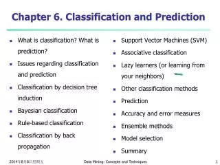
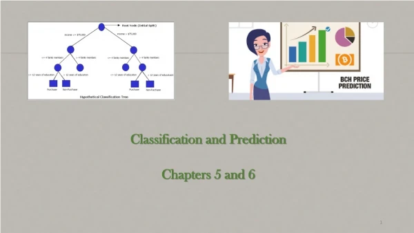
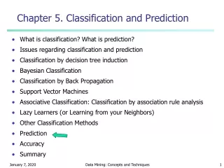
Chapter 5. Classification and Prediction • What is classification? What is prediction? • Issues regarding classification and prediction • Classification by decision tree induction • Bayesian Classification • Classification by Back Propagation • Support Vector Machines • Associative Classification: Classification by association rule analysis • Lazy Learners (or Learning from your Neighbors) • Other Classification Methods • Prediction • Accuracy • Summary Data Mining: Concepts and Techniques
Simple Linear Regression • Simple Linear Regression Model • Least Squares Method • Coefficient of Determination • Model Assumptions • Testing for Significance • Using the Estimated Regression Equation for Estimation and Prediction • Computer Solution • Residual Analysis: Validating Model Assumptions • Residual Analysis: Outliers and Influential Observations Data Mining: Concepts and Techniques
What Is Prediction? • Prediction is similar to classification • First, construct a model • Second, use model to predict unknown value • Major method for prediction is regression • Linear and multiple regression • Non-linear regression • Prediction is different from classification • Classification refers to predict categorical class label • Prediction models continuous-valued functions Data Mining: Concepts and Techniques
Predictive Modeling in Databases • Predictive modeling: Predict data values or construct generalized linear models based on the database data. • One can only predict value ranges or category distributions • Method outline: • Minimal generalization • Attribute relevance analysis • Generalized linear model construction • Prediction • Determine the major factors which influence the prediction • Data relevance analysis: uncertainty measurement, entropy analysis, expert judgement, etc. • Multi-level prediction: drill-down and roll-up analysis Data Mining: Concepts and Techniques
Regress Analysis and Log-Linear Models in Prediction • Linear regression: Y = 0 + 1 X • Two parameters , 0 and 1 specify the line and are to be estimated by using the data at hand. • using the least squares criterion to the known values of Y1, Y2, …, X1, X2, …. • Multiple regression: Y = b0 + b1 X1 + b2 X2. • Many nonlinear functions can be transformed into the above. • Log-linear models: • The multi-way table of joint probabilities is approximated by a product of lower-order tables. • Probability: p(a, b, c, d) = ab acad bcd Data Mining: Concepts and Techniques
The Simple Linear Regression Model • Simple Linear Regression Model y = 0 + 1x+ • Simple Linear Regression Equation E(y) = 0 + 1x • Estimated Simple Linear Regression Equation y = b0 + b1x ^ Data Mining: Concepts and Techniques
Simple Linear Regression Model The population regression model: Random Error term Population SlopeCoefficient Population Y intercept Independent Variable Dependent Variable Linear component Random Error component Data Mining: Concepts and Techniques
Simple Linear Regression Model (continued) Y Observed Value of Y for Xi εi Slope = β1 Predicted Value of Y for Xi Random Error for this Xi value Intercept = β0 X Xi Data Mining: Concepts and Techniques
Simple Linear Regression Equation The simple linear regression equation provides an estimate of the population regression line Estimated (or predicted) y value for observation i Estimate of the regression intercept Estimate of the regression slope Value of x for observation i The individual random error terms ei have a mean of zero Data Mining: Concepts and Techniques
Least Squares Estimators • b0 and b1 are obtained by finding the values of b0 and b1 that minimize the sum of the squared differences between y and : Differential calculus is used to obtain the coefficient estimators b0 and b1 that minimize SSE Data Mining: Concepts and Techniques
Least Squares Estimators (continued) • The slope coefficient estimator is • And the constant or y-intercept is • The regression line always goes through the mean x, y Data Mining: Concepts and Techniques
Finding the Least Squares Equation • The coefficients b0 and b1 , and other regression results in this chapter, will be found using a computer • Hand calculations are tedious • Statistical routines are built into Excel • Other statistical analysis software can be used Data Mining: Concepts and Techniques
Model Assumptions • Assumptions About the Error Term • The error is a random variable with mean of zero. • The variance of , denoted by 2, is the same for all values of the independent variable. • The values of are independent. • The error is a normally distributed random variable. Data Mining: Concepts and Techniques
Linear Regression Model Assumptions • The true relationship form is linear (Y is a linear function of X, plus random error) • The error terms, εi are independent of the x values • The error terms are random variables with mean 0 and constant variance, σ2 (the constant variance property is called homoscedasticity) • The random error terms, εi, are not correlated with one another, so that Data Mining: Concepts and Techniques
Interpretation of the Slope and the Intercept • b0 is the estimated average value of y when the value of x is zero (if x = 0 is in the range of observed x values) • b1 is the estimated change in the average value of y as a result of a one-unit change in x Data Mining: Concepts and Techniques
Simple Linear Regression Example • A real estate agent wishes to examine the relationship between the selling price of a home and its size (measured in square feet) • A random sample of 10 houses is selected • Dependent variable (Y) = house price in $1000s • Independent variable (X) = square feet Data Mining: Concepts and Techniques
Sample Data for House Price Model Data Mining: Concepts and Techniques
Graphical Presentation • House price model: scatter plot Data Mining: Concepts and Techniques
Regression Using Excel • Tools / Data Analysis / Regression Data Mining: Concepts and Techniques
Excel Output The regression equation is: Data Mining: Concepts and Techniques
Graphical Presentation • House price model: scatter plot and regression line Slope = 0.10977 Intercept = 98.248 Data Mining: Concepts and Techniques
Interpretation of the Intercept, b0 • b0 is the estimated average value of Y when the value of X is zero (if X = 0 is in the range of observed X values) • Here, no houses had 0 square feet, so b0 = 98.24833 just indicates that, for houses within the range of sizes observed, $98,248.33 is the portion of the house price not explained by square feet Data Mining: Concepts and Techniques
Interpretation of the Slope Coefficient, b1 • b1 measures the estimated change in the average value of Y as a result of a one-unit change in X • Here, b1 = .10977 tells us that the average value of a house increases by .10977($1000) = $109.77, on average, for each additional one square foot of size Data Mining: Concepts and Techniques
Example: Reed Auto Sales • Simple Linear Regression Reed Auto periodically has a special week-long sale. As part of the advertising campaign Reed runs one or more television commercials during the weekend preceding the sale. Data from a sample of 5 previous sales are shown below. Number of TV AdsNumber of Cars Sold 1 14 3 24 2 18 1 17 3 27 Data Mining: Concepts and Techniques
Example: Reed Auto Sales • Slope for the Estimated Regression Equation b1 = 220 - (10)(100)/5 = 5 24 - (10)2/5 • y-Intercept for the Estimated Regression Equation b0 = 20 - 5(2) = 10 • Estimated Regression Equation y = 10 + 5x ^ Data Mining: Concepts and Techniques
Example: Reed Auto Sales • Scatter Diagram Data Mining: Concepts and Techniques
Measures of Variation • Total variation is made up of two parts: Total Sum of Squares Regression Sum of Squares Error Sum of Squares where: = Average value of the dependent variable yi = Observed values of the dependent variable i = Predicted value of y for the given xi value Data Mining: Concepts and Techniques
Measures of Variation (continued) • SST = total sum of squares • Measures the variation of the yi values around their mean, y • SSR = regression sum of squares • Explained variation attributable to the linear relationship between x and y • SSE = error sum of squares • Variation attributable to factors other than the linear relationship between x and y Data Mining: Concepts and Techniques
Measures of Variation (continued) Y yi y SSE= (yi-yi )2 _ SST=(yi-y)2 _ y _ SSR = (yi -y)2 _ y y X xi Data Mining: Concepts and Techniques
Coefficient of Determination, R2 • The coefficient of determination is the portion of the total variation in the dependent variable that is explained by variation in the independent variable • The coefficient of determination is also called R-squared and is denoted as R2 note: Data Mining: Concepts and Techniques
Examples of Approximate r2 Values Y r2 = 1 Perfect linear relationship between X and Y: 100% of the variation in Y is explained by variation in X X r2 = 1 Y X r2 = 1 Data Mining: Concepts and Techniques
Examples of Approximate r2 Values Y 0 < r2 < 1 Weaker linear relationships between X and Y: Some but not all of the variation in Y is explained by variation in X X Y X Data Mining: Concepts and Techniques
Examples of Approximate r2 Values r2 = 0 Y No linear relationship between X and Y: The value of Y does not depend on X. (None of the variation in Y is explained by variation in X) X r2 = 0 Data Mining: Concepts and Techniques
Excel Output 58.08% of the variation in house prices is explained by variation in square feet Data Mining: Concepts and Techniques
Correlation and R2 • The coefficient of determination, R2, for a simple regression is equal to the simple correlation squared Data Mining: Concepts and Techniques
The Correlation Coefficient • Sample Correlation Coefficient where: b1 = the slope of the estimated regression equation Data Mining: Concepts and Techniques
Example: Reed Auto Sales • Sample Correlation Coefficient The sign of b1 in the equation is “+”. rxy = +.9366 Data Mining: Concepts and Techniques
Estimation of Model Error Variance • An estimator for the variance of the population model error is • Division by n – 2 instead of n – 1 is because the simple regression model uses two estimated parameters, b0 and b1, instead of one is called the standard error of the estimate Data Mining: Concepts and Techniques
Excel Output Data Mining: Concepts and Techniques
Comparing Standard Errors se is a measure of the variation of observed y values from the regression line Y Y X X The magnitude of se should always be judged relative to the size of the y values in the sample data i.e., se = $41.33K ismoderately small relative to house prices in the $200 - $300K range Data Mining: Concepts and Techniques
Inferences About the Regression Model • The variance of the regression slope coefficient (b1) is estimated by where: = Estimate of the standard error of the least squares slope = Standard error of the estimate Data Mining: Concepts and Techniques
Excel Output Data Mining: Concepts and Techniques
Comparing Standard Errors of the Slope is a measure of the variation in the slope of regression lines from different possible samples Y Y X X Data Mining: Concepts and Techniques
Inference about the Slope: t Test • t test for a population slope • Is there a linear relationship between X and Y? • Null and alternative hypotheses H0: β1 = 0 (no linear relationship) H1: β1 0 (linear relationship does exist) • Test statistic where: b1 = regression slope coefficient β1 = hypothesized slope sb1 = standard error of the slope Data Mining: Concepts and Techniques
Inference about the Slope: t Test (continued) Estimated Regression Equation: The slope of this model is 0.1098 Does square footage of the house affect its sales price? Data Mining: Concepts and Techniques
H0: β1 = 0 H1: β1 0 Inferences about the Slope: tTest Example b1 From Excel output: t Data Mining: Concepts and Techniques
H0: β1 = 0 H1: β1 0 Inferences about the Slope: tTest Example (continued) Test Statistic: t = 3.329 b1 t From Excel output: d.f. = 10-2 = 8 t8,.025 = 2.3060 Decision: Conclusion: Reject H0 a/2=.025 a/2=.025 There is sufficient evidence that square footage affects house price Reject H0 Do not reject H0 Reject H0 tn-2,α/2 -tn-2,α/2 0 -2.3060 2.3060 3.329 Data Mining: Concepts and Techniques
H0: β1 = 0 H1: β1 0 Inferences about the Slope: tTest Example (continued) P-value = 0.01039 P-value From Excel output: This is a two-tail test, so the p-value is P(t > 3.329)+P(t < -3.329) = 0.01039 (for 8 d.f.) Decision: P-value < α so Conclusion: Reject H0 There is sufficient evidence that square footage affects house price Data Mining: Concepts and Techniques
Confidence Interval Estimate for the Slope Confidence Interval Estimate of the Slope: d.f. = n - 2 Excel Printout for House Prices: At 95% level of confidence, the confidence interval for the slope is (0.0337, 0.1858) Data Mining: Concepts and Techniques
Confidence Interval Estimate for the Slope (continued) Since the units of the house price variable is $1000s, we are 95% confident that the average impact on sales price is between $33.70 and $185.80 per square foot of house size This 95% confidence interval does not include 0. Conclusion: There is a significant relationship between house price and square feet at the .05 level of significance Data Mining: Concepts and Techniques