Download
1 / 88
880 likes | 1.02k Views
Constraint Program Solvers. Generalize SAT solvers. Try to generalize systematic SAT solvers. Note: Straightforward to generalize the stochastic ones. Recall SAT enhancements to backtracking search: Careful variable ordering When we instantiate a var, shorten other clauses

E N D
Constraint Program Solvers 600.325/425 Declarative Methods - J. Eisner
Generalize SAT solvers • Try to generalize systematic SAT solvers. • Note: Straightforward to generalize the stochastic ones. • Recall SAT enhancements to backtracking search: • Careful variable ordering • When we instantiate a var, shorten other clauses • May detect conflicts • May result in unit clauses, instantiating other vars:can propagate those immediately (“unit propagation”) • Conflict analysis when forced to backtrack • Backjumping • Clause learning • Improved variable ordering 600.325/425 Declarative Methods - J. Eisner
Andrew Moore’s animations Graph coloring: Color every vertex so that adjacent vertices have different colors. (NP-complete, many applications such as register allocation) http://www-2.cs.cmu.edu/~awm/animations/constraint/ 600.325/425 Declarative Methods - J. Eisner
A few of the many propagation techniques Simple backtracking Adaptive consistency (variable elimination) All search, no propagation Good tradeoff for your problem? All propagation, no search (propagate first, then do “backtrack-free” search) 600.325/425 Declarative Methods - J. Eisner
A few of the many propagation techniques Simple backtracking (no propagation) Forward checking (reduces domains) Arc consistency (reduces domains & propagates)(limited versions include unit propagation, bounds propagation) i-consistency (fuses constraints) Adaptive consistency (variable elimination) commonly chosen 600.325/425 Declarative Methods - J. Eisner
Arc consistency (= 2-consistency) This example is more interesting than graph coloring or SAT: The < constraint (unlike in graph coloring) allows propagation before we know any var’s exact value. X must be < some Y, so can’t be 3. Hence we can propagate before we start backtracking search. (In SAT, we could only do that if original problem had unit clauses.) X Y propagation completely solved the problem! No further search necessary (this time). 1, 2, 3 1, 2, 3 X, Y, Z, T :: 1..3 X # Y Y #= Z T # Z X #< T Note: These steps can occur in somewhat arbitrary order = 1, 2, 3 1, 2, 3 T Z 600.325/425 Declarative Methods - J. Eisner slide thanks to Rina Dechter (modified)
Arc consistency is the result of “joining” binary and unary constraints X Y 1, 2, 3 1, 2, 3 … Y::1..3 … (X #< Y is an infinite table of possible vals, not shown in full) … … X::1..3 X #< Y 600.325/425 Declarative Methods - J. Eisner
really a database joinof the 3 constraints,on columns X and Y (their common vars) Arc consistency is the result of “joining” binary and unary constraints X Y 1, 2, 3 1, 2, 3 … Y::1..3 … Create table of all (X,Y) that are consistent among all 3 constraints … … X::1..3 X #< Y and X::1..3 and Y::1..3 600.325/425 Declarative Methods - J. Eisner
2 2 Arc consistency is the result of “joining” binary and unary constraints X Y These inferred restrictions to X, Y now propagate further through other constraints … 1, 2, 3 1, 2, 3 … Y::1..3 … Project those restricted values back to strengthen the unary constraints. E.g., Y=1 is not consistent with any X value, so kill it off. … … X::1..3 X #< Y and X::1..3 and Y::1..3 600.325/425 Declarative Methods - J. Eisner
Another example: Graph coloring(1,2,3 = blue, red, black) X Y 1, 2, 3 1, 2, 3 … Y::1..3 … … … X::1..3 X #\= Y 600.325/425 Declarative Methods - J. Eisner
Another example: Graph coloring(1,2,3 = blue, red, black) X Y 1, 2, 3 1, 2, 3 … Y::1..3 … No effect yet on X, Y domains. But suppose other propagations reduce X’s domain to 2 … … … X::1..3 X #\= Y and X::1..3 and Y::1..3 600.325/425 Declarative Methods - J. Eisner
Another example: Graph coloring(1,2,3 = blue, red, black) X Y 1, 2, 3 1, 2, 3 … Y::1..3 … But suppose other propagations now reduce X’s domain to 2 … … … X::2 X #\= Y and X::2 and Y::1..3 600.325/425 Declarative Methods - J. Eisner
Another example: Graph coloring(1,2,3 = blue, red, black) X Y 1, 2, 3 1, 2, 3 [1,3] … Y::1..3 … But suppose other propagations reduce X’s domain to 2 … we find Y 2. … … X::2 X #\= Y and X::2 and Y::1..3 600.325/425 Declarative Methods - J. Eisner
Another example: Graph coloring(1,2,3 = blue, red, black) X Y 1, 2, 3 1, 2, 3 [1,3] … Y::1..3 … Standard algorithm “AC-3”: Whenever X changes, construct this (X,Y) grid and see what values of Y appear on at least one green square. Here only Y=1 and Y=3 appear. … … X::2 X #\= Y and X::2 and Y::1..3 600.325/425 Declarative Methods - J. Eisner
AC-3: if X’s domain changes, recompute Y’s domain from scratch (“variable granularity”) AC-4: if X’s domain loses a particular value, reduce support for particular values in Y’s domain (“value granularity”) (there’s some recent work on speeding this up with the “watched variable” trick here) Another example: Graph coloring(1,2,3 = blue, red, black) X Y 1, 2, 3 1, 2, 3 [1,3] … Y::1..3 … Theoretically more efficient algorithm “AC-4”: Maintain the grid. Remember how many green squares are in the Y=2 column. When this counter goes to 0, conclude Y2. … … X::2 X #\= Y and X::2 and Y::1..3 600.325/425 Declarative Methods - J. Eisner
Another example: Simplified magic square • Ordinary magic square uses alldifferent numbers 1..9 • But for simplicity, let’s allow each var to be 1..3 600.325/425 Declarative Methods - J. Eisner slide thanks to Andrew Moore (modified): http://www.cs.cmu.edu/~awm/tutorials
Another example: Simplified magic square Not actually a binary constraint; basically we can keep our algorithm, but it’s now called “generalized” arc consistency. • [V1, V2, … V9] :: 1..3 • V1 + V2 + V3 #= 6, etc. 600.325/425 Declarative Methods - J. Eisner slide thanks to Andrew Moore (modified): http://www.cs.cmu.edu/~awm/tutorials
Propagate on Semi-magic Square • No propagation possible yet • So start backtracking search here 600.325/425 Declarative Methods - J. Eisner slide thanks to Andrew Moore (modified): http://www.cs.cmu.edu/~awm/tutorials
now generalized arc consistency kicks in! Propagate on Semi-magic Square • So start backtracking search here 600.325/425 Declarative Methods - J. Eisner slide thanks to Andrew Moore (modified): http://www.cs.cmu.edu/~awm/tutorials
Propagate on Semi-magic Square • So start backtracking search here any further propagation from these changes? 600.325/425 Declarative Methods - J. Eisner slide thanks to Andrew Moore (modified): http://www.cs.cmu.edu/~awm/tutorials
Propagate on Semi-magic Square • So start backtracking search here any further propagation from these changes? yes … 600.325/425 Declarative Methods - J. Eisner slide thanks to Andrew Moore (modified): http://www.cs.cmu.edu/~awm/tutorials
Propagate on Semi-magic Square • So start backtracking search here • That’s as far as we can propagate, so try choosing a value here 600.325/425 Declarative Methods - J. Eisner slide thanks to Andrew Moore (modified): http://www.cs.cmu.edu/~awm/tutorials
Propagate on Semi-magic Square • So start backtracking search here • That’s as far as we can propagate, so try choosing a value here… more propagation kicks in! 600.325/425 Declarative Methods - J. Eisner slide thanks to Andrew Moore (modified): http://www.cs.cmu.edu/~awm/tutorials
Search tree with propagation In fact, we never have to consider these if we stop at first success 600.325/425 Declarative Methods - J. Eisner slide thanks to Andrew Moore (modified): http://www.cs.cmu.edu/~awm/tutorials
So how did generalized arc consistency (non-binary constraint) work just now? a cube of (X,Y,Z) triples X+Y+Z=6 is equation of a plane through it … Y=3 Y=2 … Y=1 X + Y + Z #= 6 600.325/425 Declarative Methods - J. Eisner
So how did generalized arc consistency (non-binary constraint) work just now? … Y=3 Y=2 … … Y=1 X::1..3 X + Y + Z #= 6and [X,Y,Z]::1..3 600.325/425 Declarative Methods - J. Eisner
So how did generalized arc consistency (non-binary constraint) work just now? no values left in this plane:so grid shows that no (X,1,Z) satisfies all 3 constraints … Y=3 Y=2 no longer possible! … … Y=1 X #= 1 (assignedduring search) X + Y + Z #= 6 and X #= 1 and [Y,Z]::1..3 600.325/425 Declarative Methods - J. Eisner
So how did generalized arc consistency (non-binary constraint) work just now? no longer possible! … Z=1 Y=3 Y=2 no longer possible! … … Y=1 X #= 1 (assignedduring search) X + Y + Z #= 6 and X #= 1 and [Y,Z]::1..3 600.325/425 Declarative Methods - J. Eisner
How do we compute the new domains in practice? AC-3 algorithm from before: Nested loop over all (X,Y,Z) triples with X#=1, Y::1..3, Z::1..3 See which ones satisfy X+Y+Z #= 6 (green triples) Remember which values of Y, Z occurred in green triples no longer possible! … Y=3 Y=2 no longer possible! … … Y=1 X #= 1 (assignedduring search) X + Y + Z #= 6 and X #= 1 and [Y,Z]::1..3 600.325/425 Declarative Methods - J. Eisner
no longer possible! How do we compute the new domains in practice? Another option: Reason about the constraints symbolically! X #= 1 and X+Y+Z #= 6 1+Y+Z #= 6 Y+Z #= 5 We inferred a new constraint! Use it to reason further: Y+Z #=5 and Z #<= 3 Y #>= 2 … Y=3 Y=2 … … Y=1 X #= 1 (assignedduring search) X + Y + Z #= 6 and X #= 1 and [Y,Z]::1..3 600.325/425 Declarative Methods - J. Eisner
How do we compute the new domains in practice? Our inferred constraint X + Y #= 5 restricts (X,Y) to pairs that appear in the 3-D grid (this is stronger than individually restricting X, Y to values that appear in the grid) … Y=3 Y=2 … … Y=1 X #= 1 (assignedduring search) X + Y + Z #= 6 and X #= 1 and [Y,Z]::1..3 600.325/425 Declarative Methods - J. Eisner
How do we compute the new domains in practice? Another option: Reason about the constraints symbolically! X #= 1 and X+Y+Z #= 6 1+Y+Z #= 6 Y+Z #= 5 That’s exactly what we did for SAT: ~X and (X v Y v ~Z v W) (Y v ~Z v W) (we didn’t loop over all values of Y, Z, W to figure this out) … Y=3 Y=2 … … Y=1 X #= 1 (assignedduring search) X + Y + Z #= 6 and X #= 1 and [Y,Z]::1..3 600.325/425 Declarative Methods - J. Eisner
How do we compute the new domains in practice? Another option: Reason about the constraints symbolically! X #= 1 and X+Y+Z #= 6 1+Y+Z #= 6 Y+Z #= 5 That’s exactly what we did for SAT: ~X and (X v Y v ~Z v W) (Y v ~Z v W) • Symbolic reasoning can be more efficient:X #< 40 and X+Y #= 100 Y #> 60 (vs. iterating over a large number of (X,Y) pairs) • But requires the solver to know stuff like algebra! • Use “constraint handling rules” to symbolically propagate changes in var domains through particular types of constraints • E.g., linear constraints: 5*X + 3*Y - 8*Z #>= 75 • E.g., boolean constraints: X v Y v ~Z v W • E.g., alldifferent constraints: alldifferent(X,Y,Z) – come back to this 600.325/425 Declarative Methods - J. Eisner
Strong and weak propagators • Designing good propagators (constraint handling rules) • a lot of the “art” of constraint solving • the subject of the rest of the lecture • Weak propagators run fast, but may not eliminate all impossible values from the variable domains. • So backtracking search must consider & eliminate more values. • Strong propagators work harder – not always worth it. • Use “constraint handling rules” to symbolically propagate changes in var domains through particular types of constraints • E.g., linear constraints: 5*X + 3*Y - 8*Z #>= 75 • E.g., boolean constraints: X v Y v ~Z v W • E.g., alldifferent constraints: alldifferent(X,Y,Z) – come back to this 600.325/425 Declarative Methods - J. Eisner
B y Multiply: -7B -7y Add to: 7B + 3D > 50 Result: 3D > 50-7y Therefore: D > (50-7y)/3 Example of weak propagators:Bounds propagation for linear constraints • [A,B,C,D] :: 1..100 • A #\= B (inequality) • B + C #= 100 • 7*B + 3*D #> 50 Might want to use a simple, weak propagator for these linear constraints:Revise C, D only if something changes B’s total range min(B)..max(B). If we learn that B x, for some const x, conclude C 100-x If we learn that B y, conclude C 100-y and D > (50+7y)/3 So new lower/upper bounds on B give new bounds on C, D. That is, shrinking B’s range shrinks other variables’ ranges. 600.325/425 Declarative Methods - J. Eisner
our bounds propagator doesn’t try to get these revisions. Example of weak propagators:Bounds propagation for linear constraints • [A,B,C,D] :: 1..100 • A #\= B (inequality) • B + C #= 100 • 7*B + 3*D #> 50 Might want to use a simple, weak propagator for these linear constraints:Revise C, D only if something changes B’s total range min(B)..max(B). Why is this only a weak propagator? It does nothing if B gets a hole in the middle of its range. • Suppose we discover or guess that A=75 • Full arc consistency would propagate as follows: • domain(A) changed – revise B :: 1..100 [1..74, 76..100] • domain(B) changed – revise C :: 1..100 [1..24, 26..100] • domain(B) changed – revise D :: 1..100 1..100 (wasted time figuring out there was no change) 600.325/425 Declarative Methods - J. Eisner
Bounds propagation can be pretty powerful … • sqr(X) $= 7-X (remember #= for integers, $= for real nums) • Two solutions: • ECLiPSe internally introduces a variable Y for the intermediate quantity sqr(X): • Y $= sqr(X) hence Y $>= 0 by a rule for sqr constraints • Y $= 7-X hence X $<= 7 by bounds propagation • That’s all the propagation, so must do backtracking search. • We could try X=3.14 as usual by adding new constraint X$=3.14 • But we can’t try each value of X in turn – too many options! • So do domain splitting: try X $>= 0, then X $< 0. • Now bounds propagation homes in on the solution! (next slide) 600.325/425 Declarative Methods - J. Eisner
Bounds propagation can be pretty powerful … • Y $= sqr(X) hence Y 0 • Y $= 7-X hence X 7 by bounds propagation • X $>= 0 assumed by domain splitting during search hence Y 7 by bounds propagation on Y $= 7-X hence X 2.646 by bounds prop. on Y $= sqr(X) (using a rule for sqr that knows how to take sqrt) hence Y 4.354 by bounds prop. on Y $= 7-X hence X 2.087 by bounds prop. on Y $= sqr(X) (since we already have X 0) hence Y 4.913 by bounds prop. on Y $= 7-X hence X 2.217 by bounds prop. on Y $= sqr(X) hence Y 4.783 by bounds prop. on Y $= 7-X hence X 2.187 by bounds prop. on Y $= sqr(X) (since we already have X 0) • At this point we’ve got X :: 2.187 .. 2.217 • Continuing will narrow in on X = 2.193 by propagation alone! 600.325/425 Declarative Methods - J. Eisner
X -4 X < -4 Bounds propagation can be pretty powerful … • Y $= sqr(X),Y $= 7-X,locate([X], 0.001). % like “labeling” for real vars; % 0.001 is precision for how finely to split domain • Full search tree with (arbitrary) domain splitting and propagation: X::-..7 X 0 X < 0 X::2.193..2.193i.e., solution #1 X::-..-3.193 i.e., not done; split again! X::-..-1.810308 i.e., no solution here X::-3.193..-3.193i.e., solution #2 600.325/425 Declarative Methods - J. Eisner
Moving on … • We started with generalized arc consistency as our basic method. • Bounds consistency is weaker, but often effective (and more efficient) for arithmetic constraints. • What is stronger than arc consistency? 600.325/425 Declarative Methods - J. Eisner
etc. blue red black blue red black blue red black etc. etc. blue red black … … Looking at more than one constraint at a time • What can you conclude here? • When would you like to conclude it? • Is generalized arc consistency enough? (1 constraint at a time) blue red blue red blue red 600.325/425 Declarative Methods - J. Eisner
etc. blue red blue red alldiff blue red black alldifferent(X,Y,Z) Looking at more than one constraint at a time • What can you conclude here? • When would you like to conclude it? • Is generalized arc consistency enough? (1 constraint at a time) etc. blue red blue red blue red black X Y X Z Y Z “fuse” into bigger constraint that relates more vars at once; then do generalized arc consistency as usual. What does that look like here? 600.325/425 Declarative Methods - J. Eisner
The big fused constraint has stronger effect than little individual constraints blue red blue red alldiff blue red black red black Z=black no longer possible! Z=red no longer possible! … Z=blue alldifferent(X,Y,Z) and [X,Y]::[blue,red] and Z::[blue,red,black] 600.325/425 Declarative Methods - J. Eisner
a 4-dimensional grid showing possible values of the 4-tuple (A,B,C,D). Joining constraints in general • In general, can fuse several constraints on their common vars. • Obtain a mega-constraint. XY, XZ, YZ on the last slide happened to join into what we call alldifferent(X,Y,Z). But in general, this mega-constraint won’t have a nice name. It’s just a grid of possibilities. 600.325/425 Declarative Methods - J. Eisner
a 4-column table listing possible values of the 4-tuple (A,B,C,D). Joining constraints in general • This operation can be viewed (and implemented) as a natural join on databases. New mega-constraint. How to use it? • project it onto A axis (column) to get reduced domain for A • if desired, project onto (A,B) plane (columns) to get new constraint on (A,B) 600.325/425 Declarative Methods - J. Eisner
How many constraints should we join?Which ones? • Joining constraints gives more powerful propagators. • Maybe too powerful!: What if we join all the constraints? • We get a huge mega-constraint on all our variables. • How slow is it to propagate with this constraint(i.e., figure out the new variable domains)? • Boo! As hard as solving the whole problem, so NP-hard. • How does this interact with backtracking search? • Yay! “Backtrack-free.” • We can find a first solution without any backtracking (if we propagate again after each decision). • Combination lock again. • Regardless of variable/value ordering. • As always, try to find a good balance between propagation and backtracking search. 600.325/425 Declarative Methods - J. Eisner
Options for joining constraints(this slide uses the traditional terminology, if you care) • Traditionally, all original constraints assumed to have 2 vars • 2-consistency or arc consistency: No joining (1 constraint at a time) • 3-consistency or path consistency: Join overlapping pairs of 2-var constraints into 3-var constraints 600.325/425 Declarative Methods - J. Eisner
A note on binary constraint programs • Traditionally, all original constraints assumed to have 2 vars • Tangential question: Why such a silly assumption? • Answer: Actually, it’s completely general! (just as 3-CNF-SAT is general: you can reduce any SAT problem to 3-CNF-SAT) • You can convert any constraint program to binary form. How? • Switching variables? • No: for SAT, that got us to ternary constraints (3-SAT, not 2-SAT). • But we’re no longer limited to SAT: can go beyond boolean vars. • If you have a 3-var constraint over A,B,C, replace it with a 1-var constraint … over a variable ABC whose values are triples! • So why do we need 2-var constraints? • To make sure that ABC’s value agrees with BD’s value intheir B components. (Else easy to satisfy all the 1-var constraints!) 600.325/425 Declarative Methods - J. Eisner
5 1,2,3,4,5 5,7,11 1 2 3 4 5 3 11 9 6 7 3,6,9,12 8,9,10,11 12 10 8 9 10 11 13 12,13 10,13 12 13 transformed (“dual”) problem:one var per word, 2-var constraints. Old constraints new vars! Old vars new constraints! original (“primal”) problem:one variable per letter,constraints over up to 5 vars A note on binary constraint programs • Traditionally, all original constraints assumed to have 2 vars • If you have a 3-var constraint over A,B,C, replace it with a 1-var constraint over a variable ABC whose values are triples • Use 2-var constraints to make sure that ABC’s value agrees with BD’s value in their B components 600.325/425 Declarative Methods - J. Eisner slide thanks to Rina Dechter (modified)
Options for joining constraints(this slide uses the traditional terminology, if you care) • Traditionally, all original constraints assumed to have 2 vars • 2-consistency or arc consistency: No joining (1 constraint at a time) • 3-consistency or path consistency: Join overlapping pairs of 2-var constraints into 3-var constraints • More generally: • Generalized arc consistency: No joining (1 constraint at a time) • 2-consistency: Propagate only with 2-var constraints • 3-consistency: Join overlapping pairs of 2-var constraints into 3-var constraints, then propagate with all 3-var constraints • i-consistency: Join overlapping constraints as needed to get all mega-constraints of i variables, then propagate with those • strong i-consistency fixes a dumb loophole in i-consistency: Do 1-consistency, then 2-consistency, etc. up to i-consistency 600.325/425 Declarative Methods - J. Eisner