Download
1 / 24
250 likes | 501 Views
Running of a QED in small-angle Bhabha scattering at LEP. Introduction. QED SM are Quantum Field Theories Renormalization Running Coupling Constants QED: photon propagator Vacuum polarization charge screening Define the effective QED coupling as:

E N D
Introduction QED SM are Quantum Field Theories Renormalization Running Coupling Constants QED: photon propagator Vacuum polarization charge screening Define the effective QED coupling as: where is the fine structure constant, experimentally known to better than 410-9 is the contribution of vacuum polarization on the photon propagator, due to fermion loops In the approximation of light fermions the leading contribution is: The Leptonic contributions are calculable to very high precision The Quark contributions involve quark masses and hadronic physics at low momentum scales, not calculable with only perturbative QCD. G.Abbiendi
Dahad Optical Theorem, Dispersion Relations • Classic approach: parameterization of measured (e+e-hadrons) at low energies plus pQCD above resonances • Alternative theory-driven approaches: • pQCD applied above ≈2 GeV • pQCD in the space-like domain (via Adler function) where is smooth H.Burkhardt, B.Pietrzyk, Phys. Lett. B 513 (2001) 46 (5)had(mZ2) = 0.027610.0036 error on (5)had(mZ2) dominated by experimental errors in the energy range 1-5 GeVOne of the dominant uncertainties in the EW fits constraining the Higgs mass popular parameterization, for s>102 GeV2 or s<0 G.Abbiendi
e+ e+ a g a e- e- Small-angle Bhabha scattering an almost pure QED process. Differential cross section can be written as: Z interference correction Born term for t-channel single g exchange s-channel g exchange correction Photonic radiative corrections Effective coupling factorized a0 1/137.036 experimentally: high data statistics, very high purity This process and method advocated by Arbuzov et al., Eur.Phys.J.C 34(2004)267 G.Abbiendi
Small-angle Bhabha scattering BHLUMI MC (S.Jadach et al.) calculates the photonic radiative corrections up to O(a2L2) where L = ln ( |t| / me2 ) – 1is the Large Logarithm Higher order terms partially included through YFS exponentiation Many existing calculations have been widely cross-checked with BHLUMI to decrease the theoretical error on the determination of Luminosity at LEP, reduced down to 0.054% (0.040% due to Vacuum Polarization) Size of the photonic radiative corrections (w.r.t. Born = 1) First incomplete terms O(a2L) O(a3L3) G.Abbiendi
EL RLL e+ ER RRR IP z 6.2 cm 14.2 cm 2.5 m e SW - Left SW - Right Small-angle Bhabha scattering in OPAL 2 cylindrical calorimeters encircling the beam pipe at ± 2.5 m from the Interaction Point 19 Silicon layers 18 Tungsten layers Total Depth 22 X0 (14 cm) Each detector layer divided into 16 overlapping wedges Sensitive radius:6.2 – 14.2 cm, corresponding to scatteringangle of 25 – 58 mrad from the beam line G.Abbiendi
OPAL Si-W Luminometer Eur.Phys.J. C14 (2000) 373 Each Si layer has 16 detector wedges R-f geometry Each wedge 32x2 pads with size: R : 2.5 mm f: 11.25o G.Abbiendi
Event selection similar to the Luminosity selection The event sample is dominated by two cluster configurations with almost full energy back-to-back e+ and e- Isolation cuts 6.7 cm < RR, RL < 13.7 cm ER, EL > 0.5 Ebeam (ER + EL)/2 > 0.75 Ebeam |DF| < 200 mrad |DR| < 2.5 cm Definition cuts: 7.2 < R < 13.2 cm (at RIGHT or LEFT side), corresponding to2 ≤-t ≤ 6 GeV2 1 bin = 1 pad =2.5 mm Acceptance within Definition Cuts z = 246.0225 cm G.Abbiendi
Leading 1/t2 Bhabha spectrum We measure the effective slope bof the Bhabha t-spectrum b is related to the variation of the coupling by: Analysis method We compare the Radial distribution of the data (R t) with the theoretical predictions of the BHLUMI MC The small-angle Bhabha process is used to determine the Luminosity: we cannot make an absolute measurement of a(t), but look at its variation over the t range. Fit the Ratio f of data and MC with a(t) = a0 G.Abbiendi
Radial reconstruction Radial coordinate reconstruction is key to the current measurement Radial biases as small as 70 mm in the centre of the radial acceptance could mimic the expected running of a. Similarly would do a uniform metrology error of 0.5 mm at all radii. • Two complementary strategies used: • Unanchored coordinate: the reconstruction determines a radial coordinate R of incident showering particles in the Right and Left Si-W calorimeters. This is smooth, continuous, and uses a large number of pads throughout the depth of the detector, from many Si layers. It is projected onto a reference layer which is the Si layer at depth of 7 X0, close to the average longitudinal shower maximum. • Anchored coordinate: the residual bias on the reconstructed R is estimated and corrected by the anchoring procedure, which uses the inherent pad structure of the detector. It relies on the fact that, on average, the pad with maximum signal in any particular layer will contain the shower axis (sharp shower core). A correction is applied at each pad boundary in a chosen layer of the detector. G.Abbiendi
Radial coordinate anchoring Plot the transition from one pad to the other: Pad Boundary Images For any chosen pad boundary in any chosen Si layer, look at the Probability that the pad with the largest signal in that layer is above the boundary, as a function of the distance of the reconstructed shower from the nominal boundary position. Fit parameters: Roffis theobserved offsetsais thetransition width Total Net BiasdR (anchor) in the reconstructed Radius: geometric bias (due to Rf pads), depending on sa, determined at a testbeam small correction for the resolution flow G.Abbiendi
Layer 4 X0 1993-94 data Anchors dR Residual Bias on Radius below 30 mm Convert anchors to bin-by-bin acceptance corrections: for bin boundaries [Rinn, Rout] smaller than 1.0% for one-pad-wide bins G.Abbiendi
1993-94 LEFT 1993-94 RIGHT Widths Radial Resolution Transition width sa of the pad boundary images is related to the radial resolution sa depends on the amount of preshowering material About 2 X0 covering the middle portion of the SiW calorimeters due to cables and beam pipe structures. G.Abbiendi
pad boundaries in layer 10 9 8 7 6 5 4 3 2 1 cyan band: MC with a(t)a0 yellow band: MC with expected a(t) Study R coordinate in Data MC Represent graphically the main experimental challenge Check number of accepted events in data – MC while varying the inner radial cut in [7.2,13.2] cm cyan band: MC with a(t)a0 yellow band: MC with expected a(t) G.Abbiendi
Fit results Si layers from 1X0 to 6X0 are safe for anchoring choose layer 4X0 Preshowering Material L-R asymmetric choose Right side (cleaner than Left) 9 LEP1 data (and MC) subsamples to account for year, centre-of mass energy and running conditions LEP2 data not included due to narrower acceptance (extra shields for synchrotron radiation) and worse dead-material distribution Small corrections for: irreducible background from e+e- gg (-18 10-5) and for Z interference at off-peak energies (14 10-5) 9 subsamples consistent Statistical errors dominant Most important systematic errors due to anchoring and preshowering material Measured slope b 7.6 s (stat.) . 6.1 s (stat.+syst.) away from zero. G.Abbiendi
Experimental Systematic errors Dominant Error correlations within 10% of the total experimental errors (stat.+syst.) G.Abbiendi
Ref. BHLUMI O(a2L2) exp. Theoretical Uncertainties Photonic corrections Reliable determination of a(t) requires precise knowledge of radiative corrections Reference BHLUMI is O(a2L2) exponentiated: compare with Born, O(aL), O(a), and O(a3L3) vacuum polarization, Z-interference and s-channel switched off G.Abbiendi
Ref. BHLUMI O(a2L2) exp. Theoretical Uncertainties Photonic corrections Compare the ref. BHLUMI calculation with alternatives differing in the matrix element or in technical aspects only slope differences count Photonic corrections: the combination of the two independent MCs OLDBIS+LUMLOG allows to assess also the technical precision Full list summed in quadrature with the experimental errors G.Abbiendi
incompatible Results OPAL fit OPAL fit b = (726 96 70) 10-5 G.Abbiendi
Results Slope b = (726 96 70 50) 10-5 Significance:5.6s including all errors for the total running SM : 460 10-5 using the Burkhardt-Pietrzyk parameterization Most significant direct observation of the running of aQED ever achieved contributions to the slope b in our t range are predicted to be in the proportion: e : m : hadron ≈ 1 : 1 : 2.5 subtracting the precisely calculable leptonic contribution: Hadronic contribution to the running: First Direct Experimental evidencewith Significance of 3.0s including all errors G.Abbiendi
L3 and OPAL SM (BP-2001) both agree with SM small-angle: significance of the observed running is 6 s (dominated by OPAL) L3: 2 results with 3 s significance G.Abbiendi
TOPAZ Other Direct experimental observations (s-channel) g exchange dominates BUT full EW theory is needed OPAL (Theor.Unc. may be underestimated) TOPAZ Significance: 4.3 - 4.4 w.r.t. the no-running hypothesis BUT despite the large change in c.m.s. energy from TOPAZ to OPAL there is no sensitivity to the running of aQED between the measurements. G.Abbiendi
Other Direct experimental observations (t-channel) Large angle Bhabha: s-channel g exchange and Z interference both important VENUS: 102 ≤ -t ≤ 542 GeV2 and s-channel determined from Claimed Significance ≈ 4 but Theor.Unc. ≈ 0.5% → 2.0% could reduce it L3 (LEP2 data): 12.25 ≤ -t ≤ 3434 GeV2 Significance ≈ 3 dominated by Theor.Unc. ≈ 0.5 - 2.0 % G.Abbiendi
Conclusions • New OPAL result (PR407): scale dependence of the effective QED coupling measured from the angular spectrum of small-angle Bhabha scattering for negative momentum transfers 1.8 ≤ -t ≤ 6.1 GeV2 • theoretically almost ideal situation (precise calculations, t-channel dominance, almost pure QED, Z interference very small) • experimentally challenging BUT: large statistics, excellent purity, precise detector • Effective slope b 2 dDa / dlnt measured, good agreement with SM predictions • Strongest direct evidence for the running of aQED ever achieved in a single experiment, with significance above 5 s • First clear experimental evidence for the hadronic contribution to the running with significance of 3 s • Can Theory use this kind of t-channel measurements for aQED(mZ2) ? G.Abbiendi