Download
1 / 52
920 likes | 2.03k Views
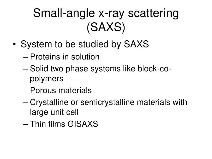
Small-angle x-ray scattering (SAXS). System to be studied by SAXS Proteins in solution Solid two phase systems like block-co-polymers Porous materials Crystalline or semicrystalline materials with large unit cell Thin films GISAXS. Solution SAXS.

E N D
Small-angle x-ray scattering (SAXS) • System to be studied by SAXS • Proteins in solution • Solid two phase systems like block-co-polymers • Porous materials • Crystalline or semicrystalline materials with large unit cell • Thin films GISAXS
Solution SAXS • The electron densities of the particles and the solution are usually assumed constant. • Then the electron density difference between the particles and the solution determines the scattering intensity. • Atomic range fluctuations in electron density are ignored. These are of course always present but do not dominate the intensity pattern.
SAXS: basics • General theory applies: I(q) = ∫ P(r) exp(i q∙r) d3r P(r) ~∫ I(q) exp(-i q∙r) d3q where P is the autocorrelation function of electron density in the sample and I(q) the intensity scattered at small angles.
Measurement • Perpendicular transmission mode • Area detector preferable • X-ray beam with small divergence • Detector with high dynamic range and low noise • Sometimes absolute intensities are needed. Obtained using a calibration sample.
SAXS: Isotropic sample • Debye equation I(q) = ΣΣ fi fj*sin(q rij)/(q rij), where fi isthe atomic scattering factor, rijthe distance of atoms i and j, and q is the magnitude of the scattering vector. • The scattering units need not to be atoms. • If continuous electron densities IN (q) =∫∫ ρ(r1)ρ(r2) sin(q r12)/(q r12) dV1dV2 wherer12=r1- r2.
One way to present the electron density of isolated particles • Let one consider a system of isolated particles in a solution. • The electron density of a particle can be presented as a product of the term ρ∞(r) of infinitely large region and the shape function σ(r) of the particle: ρ( r)=ρ∞(r)∙σ(r) • The shape functionσ(r)=1 inside the particle and 0 outside.
One way to present the autocorrelation function of the electron density P(r) = ∫ρ∞(u) ρ∞(u+r) σ(u) σ (u+r) d3u = ∫V<ρ∞(u) ρ∞(u+r)>, where V is the volume limited by the shape function. • Denoting ∫σ(u) σ (u+r) d3u = VV(r). • P(r) = ∫ρ∞(u) ρ∞(u+r) VV(r) d3u • In many cases the inner structure is ignored and one is only interested on the shape of the particles.
How to describe the electron density ρ(r)? Uniformity? Core-shell particle? More complicated density function? What about soap micelle or charged particles?
Distance distribution p(r) • The distance distribution function p(r) gives the relative number of distances of two points inside the particle as a function of the distance r. • It is obtained from the intensity I(q) as p(r) = (1/2π)3 ∫ dq 4πq2 I(q) (sinqr/qr). • The limits of integration are from 0 to ∞, which means that in practice the experimental intensity has to be extrapolated to q=0.
Distance distribution function • Consider a dilute system of particles. Particles are distributed isotropically in the sample. • Intensity I(q) in terms of the distance distribution function p(r): I(q) ≈ 4π ∫p(r) sin(qr)/(qr) dr. Integration limits from 0 to infinity
P(r) and electron density • The distance distribution function p(r) is related to the density density correlation function γ(r) of the electron density by p(r) = r2 γ(r)= r2 < ∫ρ(u) ρ(u+r)du >. • For uniform electron density γ(r) = (ρ- ρ0)2γ0(r), where γ0(r) is the plain shape factor.
Example. Spherical particle • γ0(r) = 1 - (3/4)(r/R) + (1/16)(r/R)3 • R is the radius. 2R = 100 Å
Homogeneus sphere • Scattering from an uniform sphere with the electron density ρand the radius a. The scattering amplitude is • F(q) = ∫0a 4 π2 ρsin qr dr. • This integral evaluates to • F(q) = 4/3 π a3 ρ 3 (sin x –x cos x)/x3, where x = qa. • This assumption can be used at low q-values (SAXS).
Derivative of the correlation function of an uniform particle • The shape factor γ0(r) • Limit of dγ0(r)/dr when r approaches 0 gives the surface of the particle: lim dγ0(r)/dr = -ρ2 S/4. See Feigin and Svergun.
Guinier law • Consider a dilute system of particles. • Intensity may be written as I(q) =∫∫ ρ(r1)ρ(r2) sin(q r12)/(q r12) dV1dV2 • Consider small q-values and expand the term sin(q r12)/(q r12) in series I(q) =∫∫ρ(r1)ρ(r2) [1 - (1/6)(q r12)2 + …] dV1dV2 where r122 = r12 + r22 - 2 r1 r2 • Choose the center of mass of the charge distribution as an origin. I(q) = < [ρ(r)V]2 > [1 - (1/3)(qRg)2 +…], where Rg is the radius of gyration of the charge distribution ρ.
Guinier law • At small q the shape of the intensity curve is Gaussian: I(q) ≈ I(0) exp(-(1/3)(qRg)2 ) • This approximation holds for qRg << 1.
Radius of gyration • In terms of electron density Rg = ∫ ρ(r) r2 dV / ∫ ρ(r) dV • For spherical particles Rg = (3/5)1/2 R where R is the radius of the sphere. • For an ellipsoid with semiaxes a, b, and c Rg2 = (1/5)(a2 + b2 + c2) • Thin rod Rg2 = (1/12) L2, where L is the length of the rod.
Discrete case • Particles, positionsrj • Distance of particles i and j: rij = ri –rj • Rg2 = (1/z) Σzi=1<ri2> • Another form Rg2 = (1/2z2) Σzi=1 Σzj=1 <rij2> • This can be seen by writing rij = ri –rj Rg2 = (1/2z2) Σi=1 Σj=1 <ri2> + <rj2> -2<ri·rj> Σi=1 Σj=1 <ri·rj> = < Σri >< Σrj > = 0
Radius of gyration by fitting. Take logarithms of intensity and q => linear fit. I(q) ≈ I(0) exp(-1/3(qRg)2 ) lnI(q) = lnI(0) -1/3q2Rg2q2 Examples. Proteins in solution. Rg from experimental intensity
Guinier law • First thing to check when studying solutions. • No Guinier range at small q: • The system is aggregated. Then the intensity may increase strongly towards q = 0. • The system is too dense. Then the intensity may diminish at small q because of the interparticle structure factor. • The particle size varies.
Determination of Rg in practice • Concentration series to reveal effects of interparticle interferences or aggregation. • For e.g. proteins 3-30 mg/ml • Electron density between proteins in solution and the solution usually very small. • Sometimes Rg shows a linear dependence on concentration. Extrapolation to zero concentration.
Special case: intensity of homogeneous sphere at large q • I(q) = (ρ- ρ0)2 V2 [3(sinqR – qR cosqr)/(qR)3]2 • Intensity curve show maxima. • Consider large values of qR, qR >> 1. I(q) → (ρ- ρ0)2 (4π/3R3)2 9/R4 1/q4 = (ρ- ρ0)2 4π 4πR2 1/q4 • If the number of spheres is N, IN(q) = 4π (ρ- ρ0)2 S/q4 where S is the total area. This power law behaviour of intensity is known as the Porod law.
Intensity at large q • Porod law holds for also other shapes and for non-particulate two phase systems. • How behaves intensity I(q) ≈ 4π ∫ r2 γ(r) sin(qr) / (qr) dr as q approaches to infinity? • Let D be the diameter of the particle and γ(D) = 0. • Integration by parts: I(q) = - 8π/q4 γ’(0)+ 4π/q3 Dγ’(0)sin(qD) +4π/q4 [2γ’(0)+ Dγ¨(0)] cos(qD) -4π/q4 ∫[r γ(r)](3)cos(qD)dr → constant / q4 • One needs to assume thatr γ(r) has at least continuous first and second derivatives but that [r γ(r)](3) may have discontinuities. (Feigin and Svergun)
Porod law • The assumptions hold for compact particles with smooth surfaces. • The main asymptotic term of the intensity is I(q) = -8π/q4 γ’(0). • For homogeneous particles I(q) = -4π/q4 ρ2 S, where S is the surface of the particle.
Extrapolation to q=0 • For a dilute system of homogeneous particles • I(0) = N V (ρ- ρ0)2 • Extrapolation of the intensity to zero gives the volume of the particle.
Invariant Q • Q = ∫I(q) q2 dq = 2π2 γ(0) • Q is proportional to mean square density fluctuations caused by a particle. • For a homogeneous particle Q = 2π2 V ρ2
Two-phase system • Assume two phases with constant electron densities ρ and ρ0 (particles in a matrix),shape function of particles σ • Scattering amplitude F(q) = ∫ρ(r)exp(-iq·r)dV = ∫(ρ(r)- ρ0)exp(-iq·r)dV + ∫ρ0exp(-iq·r)dV If ρ(r) is constant, I(q) = (ρ- ρ0)2 ∫ σ(r) exp(-iq·r)dV . Intensity proportional to (ρ- ρ0)2.
Invariant Q • Consider SAXS from a two-phase system • Denote electron densities by ρ1 and ρ2. • Volume fractions are denoted by v1 and v2. • The invariant Q = ∫I(q) dv • For a two-phase system Q ≈ Vv1v2 (ρ1-ρ2)2 • This can be seen as follows:
Q for a two-phase system • Electron density is written as ρ(r)= ρ0 + n(r), where the mean density is ρ0 = v1ρ1 + v2ρ2= constant. • The mean deviation is assumed to be small, <n(r)> ≈ 0. • The average <n2 (r)> ≈ v1 (ρ1-ρ0)2 + v2 (ρ2-ρ0)2 • Q = ∫∫∫ ρ(u) ρ(u+r)du exp(iq·u) d3ud3qd3r • Replace ρ(r) by ρ(r)= ρ0 +n(r)
Q for two-phase system • Q = ∫∫∫ n(u) n(u+r) exp(iq·u) d3ud3qd3r • Integrate over q to obtain Q = ∫∫ n(u) n(u+r) δ(u) d3ud3r = ∫n(r)n(r) d3r = V <n2 (r)> • Estimate the fluctuation term as <n2 (r)> = (1/V) ∫[v1(r)(ρ1(r)-ρ0)2 + v2(r)(ρ2(r)-ρ0)2] d3r
Q for a two-phase system • Q/V ≈ <n2 (r)> = v1 (ρ1-ρ0)2 + v2 (ρ2-ρ0)2 • Expanding Q/V ≈ v1ρ12 + v2ρ22 - ρ02 • Insert ρ0 = v1ρ1 + v2ρ2to obtain Q/V ≈ v1 v2 (ρ1-ρ2)2
Special cases of Porod law • IN(q) ≈ 4π (ρ- ρ0)2 S/q4at large q, where S is the total area of N particles. • Sheets I(q) ≈ const /q2 • Long thin rods I(q) ≈ const /q1 • Fractals I(q) ≈ const /qa where a gives the fractal dimension of the system.
Form factors for homogeneous particles • Nice article Jan Skov Pedersen, Analysis of small-angle scattering data from colloids and polymer solutions: modeling and least squares fitting. Advances in Colloid and Interface Science 70, 1997, 171-210.
Form factor of cylinder with radius R and length L F(q) = ∫0π/2 ((2B1(qRsinα)/(qRsinα)(sin(qLcosα/2)/(qLcosα)/2)2 sinαdα, where B1isthe first order Bessel function Guinier plot for cylinder with R=10Å, L=100Å
Infinitely thin rod • F(q) = 2 Si(qL)/(qL) – 4 sin2(qL/2)(q2L2), where Si(x) = ∫0x 1/t sin t dt and L is the length.
Infinitely thin circular disk • F(q) = 2/(q2L2)(1-B1(2qR)/(qR)), where R is the radius of the disk and B1 the Bessel function of the first kind.
Flexible polymer with Gaussian statistics • F(q) = 2(exp(-u) + u - 1)/u2 where u = <Rg2>q2 and <Rg2> is the average radius of gyration squared. • <Rg2> = (Lb)/6, where L is the contour length and b is the statistical segment length.
Flexible polymers with Gaussian statistics • Intensity is proportional to F(q) = 2(exp(-u) + u - 1)/u2 where u = <Rg2>q2 and <Rg2> is the average radius of gyration squared. • <Rg2> = (Lb)/6, where L is the contour length and b is the statistical segment length.
Star polymer with Gaussian statistics • Benoit • For a star polymer with f arms F(q) = 2/(fv2)[v-[1-exp(-v)] + (f-1)/2(1-exp(-v))2], where v = u2 f/(3f-2), and u = <Rg2>q2
compact: Calmodulin with TFP and Ca2+ elongated: Calmodulin, free Protein in solution
elongated and compact calmodulin Protein in solution
Experimental difficulties • Electron density difference between proteins and solution is small. • Very accurate background subtraction needed. • Synchrotron measurements: radiation damage • Good experimental accurace also at large q-values where the intensity is small. • Shape determination: aggregation should be prevented.
Shape determination not unambiguous • Other knowledge: • crystallography • NMR • Electron microscopy • Several new studies where it was observed that the shape obtained by SAXS is consistent with cryo-EM but not with protein crystallography.