Download
1 / 63
630 likes | 728 Views
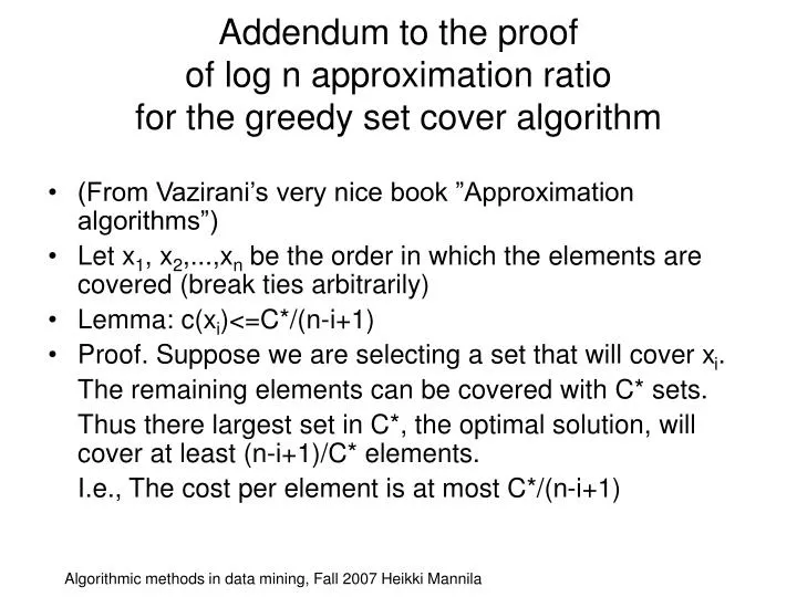
Addendum to the proof of log n approximation ratio for the greedy set cover algorithm. (From Vazirani’s very nice book ”Approximation algorithms”) Let x 1 , x 2 ,...,x n be the order in which the elements are covered (break ties arbitrarily) Lemma: c(x i )<=C*/(n-i+1)

E N D
Addendum to the proof of log n approximation ratio for the greedy set cover algorithm • (From Vazirani’s very nice book ”Approximation algorithms”) • Let x1, x2,...,xn be the order in which the elements are covered (break ties arbitrarily) • Lemma: c(xi)<=C*/(n-i+1) • Proof. Suppose we are selecting a set that will cover xi. The remaining elements can be covered with C* sets. Thus there largest set in C*, the optimal solution, will cover at least (n-i+1)/C* elements. I.e., The cost per element is at most C*/(n-i+1) Algorithmic methods in data mining, Fall 2007 Heikki Mannila
Thus • Theorem. The approximation cost is at most H(n) • Proof. The cost is at most the sum of the costs c(xi) • Proving the bound H(s) is more tedious. Algorithmic methods in data mining, Fall 2007 Heikki Mannila
Finding fragments of orders, partial orders, and total orders from 0-1 data Algorithmic methods in data mining, Fall 2007 Heikki Mannila
Themes of the chapter • Given a 0/1 a matrix • Rows: observations, columns variables • Can one find ordering information for the observations? • Without additional assumptions, no; with some assumptions, yes • Paleontological application: • find orders for subsets of fossil sites • a good ordering for (a subset of) the rows is one where the 1s are consecutive • Also other applications Algorithmic methods in data mining, Fall 2007 Heikki Mannila
Themes of the chapter • Finding small total orders (fragments) from 0-1 data • Local models/patterns • Finding partial orders from 0-1 data • A global model • Find total orders for 0-1 data • A global model Algorithmic methods in data mining, Fall 2007 Heikki Mannila
Finding small total orders (fragments) from 0-1 data • Model: a subset of observations and a total order on the subset • Task: find all such models fulfilling certain criteria • Algorithm: a pattern discovery algorithm (levelwise search) Algorithmic methods in data mining, Fall 2007 Heikki Mannila
Finding partial orders from 0-1 data • Model: a partial order over all observations • Loglikelihood: proportional to the number of cases the observed occurrence patterns violate the continuity of species • Prior: prefer partial orders that are as specific as possible • Task: find a model with high likelihood * prior • Algorithm: Find fragments and use heuristic search to build a good partial order Algorithmic methods in data mining, Fall 2007 Heikki Mannila
Find total orders for 0-1 data • Model: a total order • Loglikelihood: how many cases the observed occurrence patterns violate the continuity of species • Task: find the best total order for the observations • Algorithm: spectral method Algorithmic methods in data mining, Fall 2007 Heikki Mannila
Type of data • 0-1 data, large number of variables • Examples: • Occurrences of words in documents • Occurrences of species in paleontological sites • Occurrence of a particular motif in a promoter region of a gene • Typically the data is sparse: only a few 1s • Asymmetry between 0s and 1s • A ”1” means that there really was something • A ”0” has less information (in a way) Algorithmic methods in data mining, Fall 2007 Heikki Mannila
Example • Paleontological data from the NOW (Neogene Mammal Database) • Fossil sites (one location, one layer) • Each site contains fossils that are about the same age (+- 1 Ma) • Variables: species/genera • A ”1” is reasonably certain • A ”0” might be due to several reasons • The species was not extant at that time • The remains did not fossilize • The tooth was overlooked • … Algorithmic methods in data mining, Fall 2007 Heikki Mannila
Site-genus -matrix site genus Algorithmic methods in data mining, Fall 2007 Heikki Mannila
Background knowledge 0 0 1 1 1 0 1 0 0 1 1 • Species do not vanish and return • An ordering of the sites with a ”0” between ”1”s is improbable time Algorithmic methods in data mining, Fall 2007 Heikki Mannila
Example: seriation in paleontological data Genus • Given data about the occurrences of genera in fossil sites • Want to find an ordering in which occurrences of a genus are consecutive • Lazarus count: how many 0s are between 1s 1 1 1 0 0 0 0 0 0 0 0 0 0 0 1 1 1 1 0 1 0 0 0 1 1 1 1 0 1 0 1 1 0 1 0 1 0 0 0 0 1 1 1 1 0 0 0 0 0 0 0 0 0 0 0 1 1 1 1 0 0 0 0 0 0 0 1 1 1 1 0 1 1 1 1 1 1 0 0 0 0 1 0 1 1 0 0 0 0 0 0 0 1 1 1 1 1 1 0 0 Site Algorithmic methods in data mining, Fall 2007 Heikki Mannila
A better ordering 1 1 1 0 0 0 0 0 0 0 1 1 1 1 0 0 0 0 0 0 1 1 0 1 0 1 0 0 0 0 0 1 0 1 1 0 0 0 0 0 0 1 1 1 1 1 1 0 0 0 0 0 1 1 1 1 1 1 0 0 0 0 0 1 1 1 1 0 1 0 0 0 0 0 1 1 1 1 0 1 0 0 0 0 0 1 1 1 1 0 0 0 0 0 0 0 1 1 1 1 A smaller Lazarus count Algorithmic methods in data mining, Fall 2007 Heikki Mannila
Find small total orders (fragments) from 0-1 occurrence data • Fragment: a total ordering of a subset of observations • E.g., c<a<d<f • Intuitive interpretation: • For most variables the sequence of observations has no pattern of the form …1…0…1… 1 1 1 0 0 0 0 0 0 1 0 1 1 1 0 0 1 0 1 0 1 1 0 0 0 1 0 0 1 0 0 1 0 1 1 0 0 0 0 0 1 1 1 1 1 1 0 0 0 0 0 1 1 1 1 1 1 0 0 0 0 0 1 1 1 1 0 1 0 0 0 0 0 1 1 1 1 0 1 0 1 0 1 0 1 1 1 1 0 1 0 1 0 0 0 1 1 1 1 c a d f Algorithmic methods in data mining, Fall 2007 Heikki Mannila
Fragments of order • 0/1 data set • Fragment of order f is a sequence of observations t1 < t2 < t3 < … < tk • An variable Adisagrees with fragment f, if for some i<j<h we have ti(A)=th(A)=1, but tj(A)=0. • Otherwise t agrees with f: • Then the column for A has the form 0 0 …0 0 1 1 … 1 1 0 0 … 0 0 for the observations in f Algorithmic methods in data mining, Fall 2007 Heikki Mannila
Example a<b<c<d: dis ag dis dis 1101 0100 0101 1010 b<d<f<a: ag dis ag ag 1111 1010 1110 0011 Algorithmic methods in data mining, Fall 2007 Heikki Mannila
What is a good fragment of order? • A sequence f of rows, say, u<v<w<t • Da(f): the number of variables disagreeing with the ordering • Fr(f): the number of variables having at least 2 ones in the rows of f • A good fragment has high Fr(f) and low Da(f) Algorithmic methods in data mining, Fall 2007 Heikki Mannila
Problem statement • Given thresholds s and g • Find all fragments of order f such that in the data Fr(f) > s Da(f) < g • and all subfragments of f satisfy these • and the fragment has smaller Da value than its peers • Any other fragments from the same set of objects Algorithmic methods in data mining, Fall 2007 Heikki Mannila
Algorithm • How to find fragments with the specific properties? • Start from fragments of length 2 • No disagreements are possible • Only the bound Fr(f)>s needs to be tested • Iteration: • Assume fragments of length k-1 are known • Then we can build candidate fragments of length k • Continue until no new patterns are found • A complete algorithm: all fragments will be found Algorithmic methods in data mining, Fall 2007 Heikki Mannila
Monotonicity property • Fragment t1 < t2 < t3 < … < tkcan satisfy the requirements only if all subfragments of length k-1 satisfy them • All these have to be in the collection of fragments of size k-1 • The levelwise algorithm Algorithmic methods in data mining, Fall 2007 Heikki Mannila
Algorithm • Find F2, fragments of size 2 • C = all triples A<B<C such that A<B, A<C, and B<C are in F2 • k3 • While C is not empty compute Da(f) for all f in C Fk{f in C | Fr(f)> s and Da(f)< g } kk+1 Call fragments of length k such that all the subfragments of length k-1 are in Fk Algorithmic methods in data mining, Fall 2007 Heikki Mannila
Complexity of the algorithm • Potentially exponential in the number of variables • |F+C| = the size of the answer + all the candidates • Proportional to |F+C| n m for a matrix with n rows and m columns • Too low values of s or too high values of g will lead to huge outputs Algorithmic methods in data mining, Fall 2007 Heikki Mannila
Experimental results • Data about students and courses • Columns: students • Rows: courses • D(s,c)=1 if student s has taken course c • Here we know the true ordering • Or actually two: official ordering • Real order in which the student took the courses Algorithmic methods in data mining, Fall 2007 Heikki Mannila
Part of the recommendations Discovered fragment f Fr(f)=1361, Da(f)=3.2% Algorithmic methods in data mining, Fall 2007 Heikki Mannila
Results Algorithmic methods in data mining, Fall 2007 Heikki Mannila
Results (paleontological data) • Fragments for sites • Or transpose the matrix: fragments for species • Sequences of sites such that there are very few Lazarus events • Provide ways of looking at projections of the data • Can be used to find partial orders Algorithmic methods in data mining, Fall 2007 Heikki Mannila
Example: words in documents • Represent collections of documents as term vectors • Which words occur (1) in the document or not (0) • Very large dimensionality, lots of observations Algorithmic methods in data mining, Fall 2007 Heikki Mannila
Example from Citeseer (in 2005) What does this tell us about these terms? Databases and selectivity estimation together do not occur without queries Databases < queries < selectivity estimation Algorithmic methods in data mining, Fall 2007 Heikki Mannila
Old (2005) example from Google Scholar • prior distribution – MCMC 151,000 documents • prior distribution MCMC 2950 documents • – prior distribution MCMC 1050 documents • prior – distribution MCMC 165 documents prior < distribution < MCMC Algorithmic methods in data mining, Fall 2007 Heikki Mannila
Example from Google Scholar, Nov. 24, 2007 • prior distribution – MCMC 2,220,000 documents • prior distribution MCMC 16,300 documents • – prior distribution MCMC 6,030 documents • prior – distribution MCMC 1,230 documents prior < distribution < MCMC Algorithmic methods in data mining, Fall 2007 Heikki Mannila
An aside: have the ratios of the frequencies changed? Algorithmic methods in data mining, Fall 2007 Heikki Mannila
Next theme • Find small total orders from 0-1 data • Finding partial orders from 0-1 data • Find total orders for 0-1 data Algorithmic methods in data mining, Fall 2007 Heikki Mannila
Finding partial orders from 0-1 data • Model: a partial order over all observations • Loglikelihood: proportional to the number of cases the observed occurrence patterns violate the continuity of species • Prior: prefer partial orders that are as specific as possible • Task: find a model with high likelihood * prior • Algorithm: Find fragments and use heuristic search to build a good partial order Algorithmic methods in data mining, Fall 2007 Heikki Mannila
Why partial orders? • Determining the ages of sites is difficult • Radioisotope methods apply only to few sites • In paleontology the so-called MN system: 18 classes for the last 25 Ma • Classes are assigned by ad hoc methods • Searching for a total order might not be a good idea • The MN system is a partial order Algorithmic methods in data mining, Fall 2007 Heikki Mannila
Finding partial orders from data • How to find a partial order that fits well with the data? • What does this mean? Algorithmic methods in data mining, Fall 2007 Heikki Mannila
What is a good partial order? • The Lazarus count of a species with respect to a partial order P: • For how many sites the species was extinct at the site, but extant before and after it (as determined by P) • The same definition as for total orders • A good partial order has small Lazarus count • Can be formulated as a likelihood (a Lazarus event is a false positive) Algorithmic methods in data mining, Fall 2007 Heikki Mannila
Laz No Laz No Laz Algorithmic methods in data mining, Fall 2007 Heikki Mannila
What is a good partial order? • Find a partial order that has a low Lazarus count • The trivial partial order has Lazarus count 0 • Want to find a partial order that is specific (close to a total order) and agrees with the data • Measures of specificity: • the number of linear extensions of P (hard to compute) • number of edges in P • Find a partial order that has high specificity * likelihood Algorithmic methods in data mining, Fall 2007 Heikki Mannila
Algorithm for finding partial orders • Compute fragments from the unordered data • E.g., a < d < b < e < f and b < e < c and b < a < c < f and … • Form a precedence matrix: in what fraction of the fragments does a precede b • Form a partial order that approximates the precedence matrix (heuristic search) Algorithmic methods in data mining, Fall 2007 Heikki Mannila
Fragments and reverse fragments • The fragment generation will produce for each fragment f also its reverse fR • The pairwise precedence matrix would be useless • Divide the fragments into two classes (graph cutting) • Discard one class • Build the precedence matrix Algorithmic methods in data mining, Fall 2007 Heikki Mannila
From precedence matrix to partial order • Heuristic search • Add edges to the partial order so that the match with the precedence matrix improves • Keep track of transitivity • Difficult (and interesting) algorithmic problem • Empirical results look good • Very recent theoretical results Algorithmic methods in data mining, Fall 2007 Heikki Mannila
Algorithmic methods in data mining, Fall 2007 Heikki Mannila
Algorithmic methods in data mining, Fall 2007 Heikki Mannila
Early Miocene Transfer to late Miocene Algorithmic methods in data mining, Fall 2007 Heikki Mannila
Algorithmic methods in data mining, Fall 2007 Heikki Mannila
Themes of the talk • Find small total orders from 0-1 data • Finding partial orders from 0-1 data • Find total orders for 0-1 data Algorithmic methods in data mining, Fall 2007 Heikki Mannila
Finding good total orders for a matrix • Given a site-genus matrix • What is a good total ordering for the rows? • One in which there are as few Lazarus events as possible • Model class: total orders • Loglikelihood proportional to the number of Lazarus events Algorithmic methods in data mining, Fall 2007 Heikki Mannila
How to find such an ordering of the rows? • If there is an ordering that has no Lazarus events, it can be found in linear time (Booth & Lueker) • consecutive ones property • But normally there are (lots of) Lazarus events Algorithmic methods in data mining, Fall 2007 Heikki Mannila
Finding good total orders for a matrix • The problem of finding the best ordering of the matrix is NP-hard • Finding whether there is a submatrix of size k that has no Lazarus events is NP-hard • The fragment method finds such submatrices • Local search, traveling salesperson approaches • Spectral methods Algorithmic methods in data mining, Fall 2007 Heikki Mannila