Download
1 / 18
180 likes | 281 Views
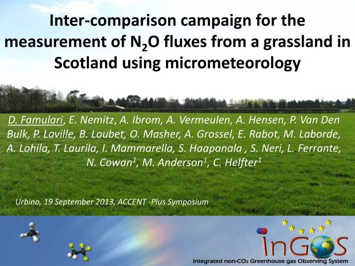
Inter-comparison campaign for the measurement of N 2 O fluxes from a grassland in Scotland using micrometeorology .

E N D
Inter-comparison campaign for the measurement of N2O fluxes from a grassland in Scotland using micrometeorology • D. Famulari, E. Nemitz, A. Ibrom, A. Vermeulen, A. Hensen, P. Van Den Bulk, P. Laville, B. Loubet, O. Masher, A. Grossel, E. Rabot, M. Laborde, A. Lohila, T. Laurila, I. Mammarella, S. Haapanala , S. Neri, L. Ferrante, N. Cowan1, M. Anderson1, C. Helfter1 Urbino, 19 September 2013, ACCENT -Plus Symposium
Objectives of the InGOSfield campaign • Improving the estimate of emission inventories for N2O using micrometeorological methods, alternative to more commonly used enclosure methods. • Standardise and improve QA/QC on non-CO2 GHG flux measurements • Give EU groups the chance to inter-compare their equipment and methods such as REA, aerodynamic gradient and eddy covariance • Introduce a protocol for the measurements of N2O Eddy Covariance (EC) fluxes. • Assess what field setup is optimum for eddy covariance • What procedures including corrections are advised in the post-processing of data
Objectives of the InGOSfield campaign • Improving the estimate of emission inventories for N2O using micrometeorological methods, alternative to more commonly used enclosure methods. • Standardise and improve QA/QC on non-CO2 GHG flux measurements • Give EU groups the chance to inter-compare their equipment and methods such as REA, aerodynamic gradient and eddy covariance • Introduce a protocol for the measurements of N2O Eddy Covariance (EC) fluxes. • Assess what field setup is optimum for eddy covariance • What procedures including corrections are advised in the post-processing of data
Field cabin setup 3 x Los Gatos Research Lasers on same absorption lines for N2O, CO and H2O Same model, but different firmware version/calibration, sample drying CW-QCL from Aerodyne Research x 2 systems: one optimised on absorption lines for CH4, N2O, H2O, the other for H2O, CO2, N2O Pulsed-QCL from Aerodyne Research optimised on absorption lines for CH4, N2O, H2O. All systems logging on a communal PC running a custom-made LabView acquisition program, able to store data synchronously from the sonic anemometers and all EC-systems at 10Hz.
Easter Bush, Edinburgh Scotland 2013 N field S field N Intensively managed grassland with a permanent meteorological field station monitoring long term EC fluxes for CO2, several years of N2O by enclosure techniques. Measurements started 3rd June 2013 and finished on 30th June 2013: first week of background measurements with sheep grazing on both fields Both fields fertilised on 11th June, with NH4NO3 (34.5% N) at a rate of 150 kg/ha Subsequent N2O emissions measured for the following 3 weeks.
Easter Bush meteorology June 2013 Easter Bush has a typical oceanic climate. In June 2013, the weather was unusually dry and sunny, with little rainfall, as a consequence of high pressure conditions.
Turbulent fluxes June 2013 Turbulent fluxes of momentum and heat were in the typical range for the Easter Bush field site, representing a fairly stable summer month.
Field setup: inlets Ultra sonic anemometers: 2 x Gill HS-50 disposed at a 90o angle, one along the fence line and one pointing into one of the fields (prevailing wind dir) Inlet tubing was 3/8” OD, different materials were used: PE, Dekabon. All lines were heated and insulated up to the analysers located indoors. One LGR system moved between 2 sonics. Flow rates: Main common inlet = 43 l/min (4 combined) DTU inlet = 30 l/min (1 system) ECN inlet = 13.7 l/min (2 system, 1 REA)
Time Response: field study Objective: Estimate the time lag and high frequency attenuation for the N2O sensors with a simple field experiment. Then compare the time lags obtained with the post-processed data by maximization of covariances method.
Cross-Calibration of all systems We used ordinary compressed air tanks as well as BOC- rated standard gas mixtures containing near-ambient levels of CH4, CO2, N2O. FTIR used as absolute value measurement, and reference to all others. The compressed gas was overflowed at the inlet end near the sonic anemometer, to let all inlets sub-sample from it.
N2O precision and stability As an outcome of the calibration exercise, an Allan variance study determines the precision at different rates of acquisition (here shown in pptV) for all systems
N2O cumulative fluxes Averaged N2O emissionsfrom 6 to 27 June 2013: onlyoverlappingmeasuringperiodswereconsidered.
Comparison of different sensors fluxes [nmol / m2 s] Each sensor (Y axes) against the “average sensor” (X axes)
Summary 6N2O eddy covariance systems have been compared during a field campaign over 25 days The N2O fast monitors were inter-calibrated via gaseous standards, and statistical analysis showed precisions ranging from 0.2 and 1 ppbV at 10Hz from 1 instance of calibration. The averaged N2O emission over the period was evaluated at 26.35 g N2O-N ha-1day-1 (EF ~1.4) With the latest generation lasers, it is possible to measure very small fluxes, potential for non-agricultural fluxes and uptake studies. Potential benefit from physically drying the sample when using CRD LGR systems All LRG systems work slightly differently (i.e. output formats, CO correction?) despite being the same model.
On-going and future work Assessment of the impact of the corrections to apply to the datasets: water effects (spectroscopic and WPL), spectral corrections Comparison of magnitude of error correction components Compilation of a wish list for field deployment and manufacturers Dataset available to the community for possible gap-filling work Comparison of three micrometeorological techniques (REA, EC, AGM), and a dynamic enclosure method. Subsets of instruments will be assessed for performance on CO2, CH4, CO, both for concentration and fluxes.