Download
1 / 22
220 likes | 352 Views
Learn about the backtracking and branch-and-bound algorithms for solving subset and permutation problems efficiently, with a focus on complexity, tree organization, and bounding functions.

E N D
Subset & Permutation Problems Subset problem of size n. Nonsystematic search of the space for the answer takes O(p2n) time, where p is the time needed to evaluate each member of the solution space. Permutation problem of size n. Nonsystematic search of the space for the answer takes O(pn!) time, where p is the time needed to evaluate each member of the solution space. Backtracking and branch and bound perform a systematic search; often taking much less time than taken by a nonsystematic search.
Tree Organization Of Solution Space • Set up a tree structure such that the leaves represent members of the solution space. • For a size n subset problem, this tree structure has 2n leaves. • For a size n permutation problem, this tree structure has n! leaves. • The tree structure is too big to store in memory; it also takes too much time to create the tree structure. • Portions of the tree structure are created by the backtracking and branch and bound algorithms as needed.
Subset Problem • Use a full binary tree that has 2n leaves. • At level i the members of the solution space are partitioned by their xivalues. • Members with xi = 1 are in the left subtree. • Members with xi = 0 are in the right subtree. • Could exchange roles of left and right subtree.
Subset Tree For n = 4 x1= 0 x1=1 x2= 0 x2=1 x2=1 x2= 0 x3=1 x3= 0 x4=1 x4=0 0001 0111 1110 1011
Permutation Problem • Use a tree that has n! leaves. • At level i the members of the solution space are partitioned by their xivalues. • Members (if any) with xi = 1 are in the first subtree. • Members (if any) with xi = 2 are in the next subtree. • And so on.
Permutation Tree For n = 3 x1= 3 x1=1 x1=2 x2= 2 x2= 3 x2= 1 x2= 3 x2= 1 x2= 2 x3=3 x3=2 x3=3 x3=1 x3=2 x3=1 123 132 213 231 312 321
Backtracking • Search the solution space tree in a depth-first manner. • May be done recursively or use a stack to retain the path from the root to the current node in the tree. • The solution space tree exists only in your mind, not in the computer.
Backtracking • The backtracking algorithm enumerates a set of partial candidates that, in principle, could be completed in various ways to give all the possible solutions to the given problem. • Backtracking is a Swiss army knife • Most problems where you can't find another solution for, are solved by backtracking
Backtracking Depth-First Search x1= 0 x1=1 x2= 0 x2=1 x2=1 x2= 0
Backtracking Depth-First Search x1= 0 x1=1 x2= 0 x2=1 x2=1 x2= 0
Backtracking Depth-First Search x1= 0 x1=1 x2= 0 x2=1 x2=1 x2= 0
Backtracking Depth-First Search x1= 0 x1=1 x2= 0 x2=1 x2=1 x2= 0
Backtracking Depth-First Search x1= 0 x1=1 x2= 0 x2=1 x2=1 x2= 0
x1= 0 x1=1 x2= 0 x2=1 x2=1 x2= 0 O(2n) Subet Sum & Bounding Functions {10, 5, 2, 1}, c = 14 Each forward and backward move takes O(1) time.
Bounding Functions • When a node that represents a subset whose sum equals the desired sum c, terminate. • When a node that represents a subset whose sum exceeds the desired sum c, backtrack. I.e., do not enter its subtrees, go back to parent node. • Keep a variable r that gives you the sum of the numbers not yet considered. When you move to a right child, check if current subset sum + r >= c. If not, backtrack.
Backtracking • Space required is O(tree height). • With effective bounding functions, large instances can often be solved. • For some problems (e.g., 0/1 knapsack), the answer (or a very good solution) may be found quickly but a lot of additional time is needed to complete the search of the tree. • Run backtracking for as much time as is feasible and use best solution found up to that time.
Branch And Bound • Search the tree using a breadth-first search (FIFObranch and bound). • Search the tree as in a bfs, but replace the FIFO queue with a stack (LIFO branch and bound). • Replace the FIFO queue with a priority queue (least-cost (or max priority) branch and bound). The priority of a node p in the queue is based on an estimate of the likelihood that the answer node is in the subtree whose root is p.
4 14 1 1 2 3 4 13 2 3 12 5 6 7 8 6 11 5 10 9 10 11 12 9 8 7 15 13 14 15 Branch And Bound • Space required is O(number of leaves). • For some problems, solutions are at different levels of the tree (e.g., 16 puzzle).
Branch And Bound • FIFO branch and bound finds solution closest to root. • Backtracking may never find a solution because tree depth is infinite (unless repeating configurations are eliminated). • Least-cost branch and bound directs the search to parts of the space most likely to contain the answer. So it could perform better than backtracking.
Branch And Bound • maintain provable lower and upper bounds on global objective value • terminate with certificate proving epsilon–sub optimality • rely on two subroutines that (efficiently) compute a lower and an upper bound on the optimal value over a given region of search space • often slow; exponential worst case performance