Download
1 / 68
680 likes | 691 Views
Chapter 5 The Searching Strategies ( Branch and bound ) ( Backtracking ) Concept: 1. Better searching (branch) method based on bound (one flexible solution) . 2. Generally, solving NP-C problems for avoiding exhaustive search . (Note: only useful in average case )

E N D
Chapter 5 The Searching Strategies (Branch and bound) (Backtracking) Concept: 1. Better searching (branch) method based onbound (one flexible solution). 2.Generally, solving NP-C problems for avoiding exhaustive search. (Note: only useful in average case) 3. Certainly, it can also solve general problems.
5-0 Concepts • Tree Searching problems • The solutions of many problems may be represented by trees. • Thus, we can solve these problems by tree searching strategy.
5-0 Satisfiability problem (See Chap 8) Tree Representation of Eight Assignments. If there are n variables x1, x2, …,xn, then there are 2n possible assignments.
5-0 Satisfiability problem (NPC) • An instance: (See: ch8: Semantic Tree) -x1……..……(1) x1…………..(2) x2 v x5….….(3) x3…….…….(4) -x2…….…….(5) A Partial Tree to Determine the Satisfiability Problem. • We may not need to examine all possible assignments. • But, all possible assignments almost need to be examined in the worst cast.
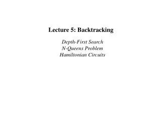
5-0 Hamiltonian circuit problem (NPC) • E.g. the Hamiltonian circuit problem: A Hamiltonian cycle is a round trip path along n edges of G=(V,E) which visits every vertexonce and returns to its starting vertex. A Graph Containing a Hamiltonian Circuit
Fig. 5-8 The Tree Representation of Whether There Exists a Hamiltonian Circuit of the Graph in Fig. 5-6
5-1 The Breadth-First Search (BFS) • Method: (A Queue can be used to guide BFS) • Traversal the tree representation by breadth-first manner and test whether it has obtained a solution. • Example: 1 2 7 5 1 1 6 3 4 2 3 4 2 6 3 3 5 6 7 8 5 2 4 9 10 11 12 13 4 4 7 5 7 5 7 3 7 4 7 6 5 6 7 6 5 5 2 3 6 2 1 1
5-2 The Depth-first search • E.g. sum of subset problem S={7, 5, 1, 2, 10} S’ S sum of S’ = 9 ? Fig. 6-11 A Sum of Subset Problem Solved by Depth-First Search. • A stackcan be used to guide the depth-first search.
5-2 The Depth-First Search (Compare with BFS in Slide 5-7) • Method: • Traversal the tree representation by depth-first manner and test whether it has obtained a solution. • Example: 1 2 7 5 1 1 6 3 4 2 2 6 3 3 3 5 2 4 4 4 4 7 5 7 5 8 5 7 3 7 4 7 6 5 6 7 6 7 6 5 5 2 3 9 10 6 11 2 1 1
5-3 Hill climbing • A variant of depth-first search The method selects the locally optimal node to expand. • E.g. 8-puzzle problem evaluation function f(n) = d(n) + w(n) , where d(n) is the depth of node n and w(n) is # of misplaced tiles in node n.
Fig. 5-15 An 8-Puzzle Problem Solved by a Hill Climbing Method f(n) = d(n) + w(n) 4 = 1 + 3 (1,2,8)
5-4 Best-first search strategy • Combing depth-first search and breadth-first search • Selecting the node with the best estimated cost among all nodes. • This method has a global view.
Fig. 5-16 An 8-Puzzle Problem Solved by a Best-First Search Scheme
5-4 Best-First Search Scheme • Step1:Form a one-element list consisting of the root node. • Step2:Remove the first element from the list. Expand the first element. If one of the descendants of the first element is a goal node, then stop; otherwise, add the descendants into the list. • Step3: Sort the entire list by the values of some estimation function. • Step4:If the list is empty, then failure. Otherwise, go to Step 2.
Summary of Searching methods • Breadth-First Search (BFS) • Depth-First Search (DFS) => Be used to judge connected graph • Hill climbing (HCS): A variant of DFS • Best-First Search (Best-FS) • How to obtain “Bound” (one flexible solution): • Using DFS, HCS or Best-FS to find it. • Graph Theory => Important
Graph Theory => Important • Graph Representation => Data structure, Discrete Math. • Famous Graph Problems A. Graph Traversals B. Connectivity C. Minimum Spanning Tree D. Shortest Path E. Maximum Flow F. Matching G. TSP H. Graph Coloring I. Vertex Cover and Independent Set
Graph Theory A E B D C • Biconnected Components(BC) • Undirected GraphG=(V,E) • G is biconnected if 2 vertex disjoint paths between each pair of vertices, or G has one edge. • G is biconnected iff it contains no articulation points. • Fault tolerance • DFS- undirected graphs have only Tree and Back edge set
A A E B E B Remove node “A” D C D C Biconnected component A A E E Remove node “B” B B D D C C Non-biconnected component Biconnected Components(BC) Definition: Articulation point “a” • A vertex “a” whose removal will split G into many parts. * B is an Art. Point : (u,v) s.t. every path between u and v contains “a”.
v1 v2 v1 v2 v4 v3 v5 v2 v3 v4 v4 v5 v6 v9 v6 v6 v9 v7 v8 v7 v8 Biconnected Components(BC) Deleting each node, to find articulation points • A biconnected component is a maximal subset of edges such that all components in its induced subgraph are biconnected.
Strongly Connected Components (SCC) Strongly Connected Components (SCC) G is strongly connected iff for every pair of vertices: u, v V, uv and vu. - A strongly connected component is a maximal subset of the vertices such that its induced subgraph is strongly connected.
G2 G G1 a b c d a b c d G3 G4 e f g h e f g h Strongly Connected Components (SCC) • Goal: Given a directed graph G=(V,E), partition G into subgraphs G1,G2,…,Gk s.t. Gi is a SCC of G. Example : partition
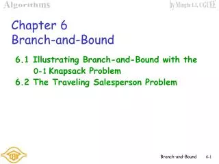
5-5 The branch-and-bound strategy • This strategy can be used to solve optimization problems. (DFS, BFS, hill climbing and best-first search can not be used to solve optimization problems.) • Remark: Using searching method to find a solution (Bound) to reduce the branch. • E.g. Fig. 5-17 A Multi-Stage Graph Searching Problem. Recall: Chap3 Greedy method cannot resolve it. Chap 7 Dynamic programming can solve it.
5-5 Solved by branch-and-bound (Solution) See Fig. 5-18, 5-19
5-5 Solved by branch-and-bound • Pre-view of branch-and-bound approach • Using lower bound • The personnel assignment problem • Branch depends on Job order • The traveling salesperson optimization problem • Branch depends on Max of min (row+column) • Using upper bound and lower bound • The 0/1 knapsack problem • Branch depends on general permutation (x1=1, x1=0)
5-6 The personnel assignment problem(Using lower bound) • A linearly ordered set of persons P={P1, P2, …, Pn} where P1<P2<…<Pn • A partially ordered set of jobs J={J1, J2, …, Jn} • Suppose that Pi and Pj are assigned to jobs f(Pi) and f(Pj) respectively. If f(Pi) f(Pj), then Pi Pj. Cost Cij is the cost (Pay) of assigning Pi to Jj. We want to find a feasible assignment with the min. cost (Pay). i.e. • Xij = 1 if Pi is assigned to Jj and Xij = 0 otherwise. • Minimize i,j CijXij
J1 J1, J2, J2 J3, J4 5-6 The personnel assignment problem ↓ J1, ↘ J2, ↓ J4, J3 J3 J4 J1, J3, J2, J4 J2, J1, J3, J4 J2, J1, J4 J3 • E.g. Fig. 5-21 A Partial Ordering of Jobs • After topological sorting, one of the following topologically sorted sequences will be generated: • P1 P2 P3 P4 • One of feasible assignments: P1→J1, P2→J2, P3→J3, P4→J4
Jobs Persons 1 2 3 4 5-6 The personnel assignment problem 1 29 19 17 12 2 32 30 26 28 3 3 21 7 9 4 18 13 10 15 • Cost matrix: Table 5-1 A Cost Matrix for a Personnel Assignment Problem
Jobs Persons 1 2 3 4 5-6 The personnel assignment problem 1 17 4 5 0 (-12) 2 6 1 0 2 (-26) 3 0 15 4 6 (-3) 4 8 0 0 5 (-10) (-3) • Reduced cost matrix: subtract a constant from each row and each column respectively such that each row and each column contains at least one zero. Table 5-2 A Reduced Cost Matrix
5-6 The personnel assignment problem • Total cost subtracted: 12+26+3+10+3 = 54 • This is a lower bound of our solution.
5-6 The personnel assignment problem • Solution tree: (Recall Slide 5-19) Job order
5-6 The personnel assignment problem • Apply the best-first search scheme: (Without reduced cost matrix)
5-6 The personnel assignment problem • Bounding of sub-solutions: (With reduced cost matrix)
j i 1 2 3 4 5 6 7 5-7 The traveling salesperson optimization problem (Using lower bound) 1 ∞ 3 93 13 33 9 57 2 4 ∞ 77 42 21 16 34 3 45 17 ∞ 36 16 28 25 4 39 90 80 ∞ 56 7 91 5 28 46 88 33 ∞ 25 57 6 3 88 18 46 92 ∞ 7 7 44 26 33 27 84 39 ∞ • It is NP-complete • E.g. cost matrix: • Table 5-3 A Cost Matrix for a Traveling Salesperson Problem.
j i 1 2 3 4 5 6 7 5-7 The traveling salesperson optimization problem 1 ∞ 0 90 10 30 6 54 (-3) 2 0 ∞ 73 38 17 12 30 (-4) 3 29 1 ∞ 20 0 12 9 (-16) 4 32 83 73 ∞ 49 0 84 (-7) 5 3 21 63 8 ∞ 0 32 (-25) 6 0 85 15 43 89 ∞ 4 (-3) 7 18 0 7 1 58 13 ∞ (-26) reduced:84 • Reduced cost matrix: Table 5-4 A Reduced Cost Matrix.
j i 1 2 3 4 5 6 7 5-7 The traveling salesperson optimization problem 1 ∞ 0 83 9 30 6 50 2 0 ∞ 66 37 17 12 26 3 29 1 ∞ 19 0 12 5 4 32 83 66 ∞ 49 0 80 5 3 21 56 7 ∞ 0 28 6 0 85 8 42 89 ∞ 0 7 18 0 0 0 58 13 ∞ (-7) (-1) (-4) Max of min( Row+Col.) for each zero element Table 5-5 Another Reduced Cost Matrix. Arc 3-5 Arc 4-6
5-7 The traveling salesperson optimization problem • Total cost reduced: 84+7+1+4 = 96 (lower bound) decision tree: Fig. 5-25 The Highest Level of a Decision Tree. • If we use arc 3-5 to split, the difference on the lower bounds is 17+1 = 18. Max of min
5-7 The traveling salesperson optimization problem Table 5-6 A Reduced Cost Matrix if Arc 4-6 is Included. (Since Arc 4-6 is included, Arc 6-4 can not be included)
j i 1 2 3 4 5 7 5-7 The traveling salesperson optimization problem 1 ∞ 0 83 9 30 50 2 0 ∞ 66 37 17 26 3 29 1 ∞ 19 0 5 5 0 18 53 4 ∞ 25 (-3) 6 0 85 8 ∞ 89 0 7 18 0 0 0 58 ∞ • The cost matrix for all solution with arc 4-6: Table 5-7 A Reduced Cost Matrix for that in Table 6-6. • Total cost reduced: 96+3 = 99 (new lower bound)
99=96+3 Fig 5-26 A Branch-and-Bound Solution of a Traveling Salesperson Problem. Because 117<126
5-8 The 0/1 knapsack problem(Using upper bound and lower bound) • Positive integer P1, P2, …, Pn (profit) W1, W2, …, Wn (weight) M (capacity)
5-8 The 0/1 knapsack problem • Fig. 5-27 The Branching Mechanism in the Branch-and-Bound Strategy to Solve 0/1 Knapsack Problem.
i 1 2 3 4 5 6 5-8 The 0/1 knapsack problem Pi 6 10 4 5 6 4 Wi 10 19 8 10 12 8 (Pi/Wi Pi+1/Wi+1), pre-sorting • E.g. n = 6, M = 34 • A feasible solution: X1 = 1, X2 = 1, X3 = 0, X4 = 0, X5 = 0, X6 = 0 -(P1+P2) = -16 (upper bound) Any solution higher than -16 can not be an optimal solution.
5-8 The 0/1 knapsack problem • Relax our restriction from Xi = 0 or 1 to 0 Xi 1 (knapsack problem)
5-8 The 0/1 knapsack problem • We can use the greedy method to find an optimal solution for knapsack problem: X1 = 1, X2 =1, X3 = 5/8, X4 = 0, X5 = 0, X6 =0 -(P1+P2+5/8P3) = -18.5 (lower bound) -18 is our lower bound. (only consider integers) -18 optimal solution -16 optimal solution: X1 = 1, X2 = 0, X3 = 0, X4 = 1, X5 = 1, X6 = 0 -(P1+P4+P5) = -17
Finishing the figure Fig. 5-28 0/1 Knapsack Problem Solved by Branch-and-Bound Strategy
5-10 The A* algorithm (Shortest path) • Used to solve optimization problems. • Using the best-first strategy. • If a feasible solution (goal node) is obtained, then it is optimal and we can stop. • Cost function of node n : f(n) f(n) = g(n) + h(n) g(n):cost from root to node n. h(n):estimated cost from node n to a goal node. h*(n):“real” cost from node n to a goal node. h(n) h*(n) f(n) = g(n) + h(n) g(n)+h*(n) = f*(n) Important concept
5-10 The A* algorithm • Stop iff the selected node is also a goal node • E.g. Fig. 5-36 A Graph to Illustrate A* Algorithm. Shortest path From S to T
5-10 The A* algorithm • Step 1. f(n) = g(n) + h(n), where g(n):cost from root to node n. h(n):estimated cost from node n to a goal node.
5-10 The A* algorithm • Step 2. Expand A ( Min f(A) )
5-10 The A* algorithm • Step 3. Expand C( Min f(C) )