Download
1 / 19
190 likes | 296 Views
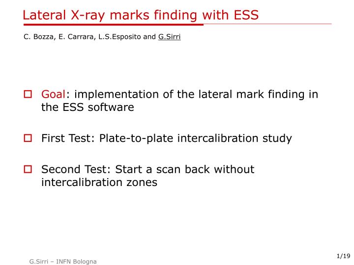
Lateral X-ray marks finding with ESS. Goal : implementation of the lateral mark finding in the ESS software First Test: Plate-to-plate intercalibration study Second Test: Start a scan back without intercalibration zones. C. Bozza, E. Carrara, L.S.Esposito and G.Sirri. Lateral X-ray mark. X.

E N D
Lateral X-ray marks finding with ESS • Goal: implementation of the lateral mark finding in the ESS software • First Test: Plate-to-plate intercalibration study • Second Test: Start a scan back without intercalibration zones C. Bozza, E. Carrara, L.S.Esposito and G.Sirri
Mark recognition Not possible to be done: • No extra camera with low magnification optics are available • Only a small amount of the lines can be scanned • The two strip are not always long enough to print a clear crossing point • Not possible to scan only one FOV per mark The approach is: • Three segments of each strip are scanned and lines are obtained by a linear fit. The coordinates of intersection point are the mark coordinates. NO NO Intersectionpoint
Mark finding procedure This is the procedure currently under test. 4. Repeat 2,3for the 2nd line 1. Set the corner 2. Scan this edge to find a first line segment 3. Scan further two line segment here 6. Evaluate the intersection points and evaluate the transformation 5. Repeat 2,3,4 for the second mark
How the transformation is evaluated? Rdet=A · Rstage +B Affine transf. of the plane are composed of scaling (reflections), rotations, and translations. Emphasizing this order, the components of a transformation can be encoded with the IFS formalism: r – scaling (reflection) in the x direction s – scaling (reflection) in the y direction theta - rotation of horizontal lines phi - rotation of vertical lines e - horizontal translation f - vertical translation With 2 mark coordinates: up to 4 independent parameter can be evaluated r=s , theta=phi , e , f (same scaling for both axis, rigid rotation, translation)
Mark finding reproducibility 5 measure of the mark coordinates without removing the emulsion plate IntersectionMark1: ( 121722.1 , 3101.5 ) ( 121722.4 , 3099.6 ) ( 121722.4 , 3107.0 ) ( 121722.4 , 3104.7 ) ( 121722.3 , 3102.8 ) IntersectionMark2: ( 121820.2 , 97942.4 ) ( 121818.3 , 97937.0 ) ( 121820.3 , 97943.1 ) ( 121822.9 , 97938.3 ) ( 121820.3 , 97936.6 ) The system is able to find the marks within 10 microns( better for the X coordinate )
First Test: plate-to-plate intercalibration study • A first test has been done by scanning 5 * 1 cm² zones in two adjacent emulsion plates of a brick exposed to cosmic rays. • The scanning was done at LNGS Scanning station with a vacuum system equipped with a vacuum channel larger than the emulsion size. Adhesive tape emulsion 3 1 glass 5 4 2 Vacuum channel • The emulsion were attached to the adhesive tape • In this setup the mark lines images are not affected by the vacuum channel image • Scanning done using the mark finding module in the acquisition sw
First Test: plate-to-plate intercalibration study • Tracks of the first plate are projected to the second one without extra intercalibration • Pattern match results: ZONE 1 DX : E: 100 M: -14.0 RMS: 8.8 ZONE 1 DY : E: 100 M: 33.0 RMS: 8.2 ZONE 2 DX : E: 51 M: -7.0 RMS: 11.6 ZONE 2 DY : E: 51 M: -3.2 RMS: 9.1 ZONE 3 DX : E: 105 M: -3.7 RMS: 8.0 ZONE 3 DY : E: 105 M: -7.6 RMS: 10.3 ZONE 4 DX : E: 86 M: 10.5 RMS: 5.6 ZONE 4 DY : E: 86 M: 13.5 RMS: 5.9 ZONE 5 DX : E: 91 M: -6.5 RMS: 7.0 ZONE 5 DY : E: 91 M: 9.4 RMS: 6.7
First Test: Evaluation of the best transformation After matching the track couples can be used to evaluate the intercalibration between the 2 plates. The results have to be compared with the Identity transformation which is the one supposed to be used without intercalibration zones. 406 matches found. QMAP – 6 parameters Aff2D : 0.999894 -0.000181 0.000207 0.999933 18.65 -20.81 (DET=0.999827) r: 0.999894 s: 0.999933 theta: 0.000207 phi: 0.000182 e : 18.65 f : -20.81 QMAP - 3 parameters (EdbAffine class implemented) Aff2D: 1.000000 -0.000199 0.000199 1.000000 12.09 -23.41 (DET=1.000000) r: 1.000000 s: 1.000000 theta: 0.000199 phi: 0.000199 e : 12.09 f : -23.41 Scaling and Rotation are very small (< 1/10000). The translation error is about 20 micron.
Second Test: start a scan back • The scan back of brick 8199 with a predicted track has been started for test. • This scanning has been done at Bologna using a vacuum system with a standard vacuum channel • To avoid interference with the image of the vacuum channel the emulsion plate was placed at the edge of the channel with lateral mark outside the vacuum area. Vacuum channel
Second Test: scan back history (5 plates) • Scan Back done without computing infrastructure assistance. Linking and Prediction Finding has done manually POS TOL = 100 micron SLOPE TOL = 0.03 + 0.05*SLOPE PL PPX PPY PSX PSY FPX FPY FSX FSY FP DPX DPY 1 -2968655 -3247649 -0.405 0.508 -2968628 -3247628 -0.388 0.506 23 -27 -21 -2968628 -3247629 -0.374 0.519 20 -27 -20 2 -2968124 -3248286 -0.388 0.506 -2968073 -3248362 -0.381 0.499 33 -51 76 3 -2967578 -3249011 -0.381 0.499 4 -2967082 -3249659 -0.381 0.499 -2967042 -3249708 -0.393 0.503 23 -41 48 5 -2966531 -3250362 -0.393 0.503 -2966546 -3250378 -0.382 0.503 24 16 16 -2966564 -3250327 -0.383 0.492 16 34 -34 • Plate 3 : not found also for the scan back with intercalibration zones • Plate 4 : skipped by the scan back with intercalibration zones because optical marks were printed on the wrong emulsion side.
Technical considerations • The sw implementation is working, but it cannot be considered in the final state. • For the version I’m testing: • “Automatic search of the First Mark” procedure not tested • The Mark Finding can fail if used above the vacuum channel • Automatic recovery strategy and manual set procedure are not implemented • No autofocus • Sometimes it recognize the (wrong) X-ray line placed ~1 mm far from each vertical strip.
How to deal with … • For these tests • Set the upper-right corner manually • Use of large vacuum area plate and attach emulsion on an adhesive tape • Use the standard but put the markers outside the vacuum area • Use precise mechanical reference on the glass plate • Put the exact emulsion sizes in the map string • Failures if marks are outside the vacuum area; set the Z with care. • Open the log file and check manually if wrong strip is recognize • The development is in progress.
Conclusions • The current implementation of the lateral mark finding in the ESS software has been tested and is working correctly (with some technical prescriptions). • Mark finding reproducibility is good • Plate-to-plate intercalibration of the order of 20 micron. • The development to have a “foolish proof” version is in progress