Download
1 / 9
100 likes | 243 Views
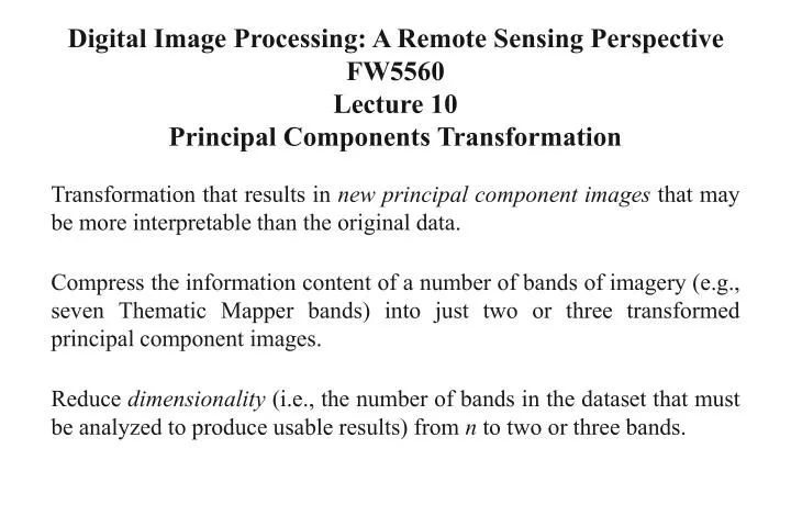
Digital Image Processing: A Remote Sensing Perspective FW5560 Lecture 10 Principal Components Transformation. Transformation that results in new principal component images that may be more interpretable than the original data.

E N D
Digital Image Processing: A Remote Sensing Perspective FW5560 Lecture 10 Principal Components Transformation Transformation that results in new principal component images that may be more interpretable than the original data. Compress the information content of a number of bands of imagery (e.g., seven Thematic Mapper bands) into just two or three transformed principal component images. Reduce dimensionality (i.e., the number of bands in the dataset that must be analyzed to produce usable results) from n to two or three bands.
The spatial relationship between the first two principal components: (a) Scatter-plot of data points collected from two remotely bands labeled X1 and X2 with the means of the distribution labeled µ1 and µ2. (b) A new coordinate system is created by shifting the axes to an X system. The values for the new data points are found by the relationship X1 = X1 – µ1 and X2 = X2 – µ2. This is a Translation (c) The X axis system is then rotated about its origin (µ1, µ2) so that PC1 is projected through the semi-major axis of the distribution of points and the variance of PC1 is a maximum. PC2 must be perpendicular to PC1 or orthogonal. The PC axes are the principal components of this two-dimensional data . This is a Rotation
The n ncovariance matrix, Cov, of the n-dimensional remote sensing data set to be transformed is computed. Use of the covariance matrix results in an unstandardized PCA., Use of the correlation matrix results in a standardized PCA.
Eigenvectors (ap) (Factor Scores) Computed for the Covariance Matrix
Eigenvalues, E= [λ1,1, λ2,2, λ3,3, …, λ n.n]. Think of theses as expressing the “variance” of the component- in other words the length of the component axis. Why are off diagonal elements = 0?
Eigenvalues Computed for the Covariance Matrix p = 1 7 p = 1
Factor Loading, Rk,p, Between Band k and Each Principal Component p where: ak,p = eigenvector for band k and component p lp = pth eigenvalue Vark = variance of band k in the covariance matrix
Compute a new value for pixel 1,1 (it has 7 bands) in principal component number 1 using the following equation: original remote sensor data for pixel 1,1 where akp= eigenvectors, BVi,j,k = brightness value in band k for the pixel at row i, column j, and n = number of bands.
Important to think about the type of transformation Scene dependent Empirical What is the difference?