Download
1 / 37
370 likes | 489 Views
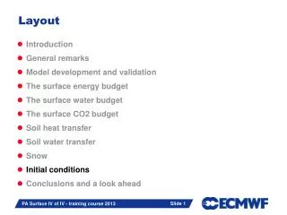
Layout. Introduction General remarks Model development and validation The surface energy budget Soil heat transfer Soil water transfer Surface water fluxes Initial conditions Snow Conclusions and a look ahead. H. LE. Day. D. Night. G.

E N D
Layout • Introduction • General remarks • Model development and validation • The surface energy budget • Soil heat transfer • Soil water transfer • Surface water fluxes • Initial conditions • Snow • Conclusions and a look ahead PA Surface II of IV - training course 2006
H LE Day D Night G Thermal budget of a ground layer at the surface PA Surface II of IV - training course 2006
Dry Fir canopy Barley field Energy budget: Summer examples Arya, 1988 PA Surface II of IV - training course 2006
Surface albedo Surface emissivity Skin temperature The surface radiation • In some cases (snow, sea ice, dense canopies) the impinging solar radiations penetrates the “ground” layer and is absorbed at a variable depth. In those cases, an extinction coefficient is needed. Arya, 1988 PA Surface II of IV - training course 2006
Sensible heat flux specify the surface Evaporation Ground heat flux The other terms PA Surface II of IV - training course 2006
Recap: The surface energy equation • Equation for • For: • a thin soil layer at the top • G (Ts,Tsk) is known, or parameterized or G << Rn we have a non-linear equation defining the skin temperature PA Surface II of IV - training course 2006
TESSEL • Skin layer at the interface between soil (snow) and atmosphere; no thermal inertia, instantaneous energy balance • At the interface soil/atmosphere, each grid-box is divided into fractions (tiles), each fraction with a different functional behaviour. The different tiles see the sameatmospheric column above and the samesoil column below. • If there are N tiles, there will be N fluxes, N skin temperatures per grid-box • There are currently up to 6 tiles over land (N=6) PA Surface II of IV - training course 2006
TESSEL skin temperature equation • Grid-box quantities PA Surface II of IV - training course 2006
Land Sea and ice High vegetation Open sea / unfrozen lakes Low vegetation Sea ice / frozen lakes High vegetation with snow beneath Snow on low vegetation Bare ground Interception layer Tiles PA Surface II of IV - training course 2006
Fields ERA15 TESSEL Vegetation Fraction Fraction of low Fraction of high Vegetation type Global constant (grass) Dominant low type Dominant high type Albedo Annual Monthly LAI rsmin Global constants Annual, Dependent on vegetation type Root depth Root profile 1 m Global constant Annual, Dependent on vegetation type TESSEL geographic characteristics PA Surface II of IV - training course 2006
High vegetation fraction at T511 (now at T799) Aggregated from GLCC 1km PA Surface II of IV - training course 2006
Low vegetation fraction at T511 (now at T799) Aggregated from GLCC 1km PA Surface II of IV - training course 2006
High vegetation type at T511 (now at T799) Aggregated from GLCC 1km PA Surface II of IV - training course 2006
Low vegetation type at T511 (now at T799) Aggregated from GLCC 1km PA Surface II of IV - training course 2006
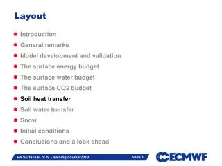
Layout • Introduction • General remarks • Model development and validation • The surface energy budget • Soil heat transfer • Soil water transfer • Surface water fluxes • Initial conditions • Snow • Conclusions and a look ahead PA Surface II of IV - training course 2006
Hillel 1982, 1998 Soil science miscellany (1) • The soil is a 3-phase system, consisting of • minerals and organic matter soil matrix • water condensate (liquid/solid) phase • moist air trapped gaseous phase • Texture - the size distribution of soil particles PA Surface II of IV - training course 2006
Soil science miscellany (2) • Structure - The spatial organization of the soil particles • Porosity - (volume of maximum air trapped)/(total volume) Hillel 1982,1998 • Composition • Water content Reference:Hillel 1998 Environmental Soil Physics, Academic Press Ed. PA Surface II of IV - training course 2006
Rosenberg et al 1983 Arya 1988 Soil properties PA Surface II of IV - training course 2006
Ground heat flux In the absence of phase changes, heat conduction in the soil obeys a Fourier law • Boundary conditions: • Top Net surface heat flux • BottomNo heat flux OR prescribed climate PA Surface II of IV - training course 2006
summer winter surface bare sod summer 50 cm depth Diurnal cycle of soil temperature Rosenberg et al 1983 PA Surface II of IV - training course 2006
TESSEL • Solution of heat transfer equation with the soil discretized in 4 layers, depths 7, 21, 72, and 189 cm. • No-flux bottom boundary condition • Heat conductivity dependent on soil water • Thermal effects of soil water phase change ↓0.1~0.6 d ↓1.1~5.8 d ↓10.6 ~ 55.8 d Time-scale for downward heat transfers in wet/dry soil PA Surface II of IV - training course 2006
TESSEL soil energy equations j-1 Gj-1/2 Tj Dj Gj+1/2 j+1 PA Surface II of IV - training course 2006
140 m 2 m Soil Case study: winter (1) Model vs observations, Cabauw, The Netherlands, 2nd half of November 1994 PA Surface II of IV - training course 2006
Observations: Numbers Model: Contour Case study: winter (2) Soil Temperature, North Germany, Feb 1996: Model (28-100 cm) vs OBS 50 cm PA Surface II of IV - training course 2006
T air G T skin LE H Rnet Case study: winter (3) Viterbo, Beljaars, Mahfouf, and Teixeira, 1999: Q.J. Roy. Met. Soc., 125,2401-2426. • Model bias: • Net radiation (Rnet) too large • Sensible heat (H) too small • But (Tair-Tsk) too large (too large diurnal cycle) • Therefore f(Ri) problem • Soil does not freeze (soil temperature drops too quickly seasonally) Stability functions Soil water freezing PA Surface II of IV - training course 2006
Apparent heat capacity Winter: Soil water freezing Soil heat transfer equation in soil freezing condition PA Surface II of IV - training course 2006
Observations Stab+Freezing Stability Control 1 Jan 1 Feb 1 Nov 1 Oct 1 Dec Case study: winter (4) Germany soil temperature: Observations vs Long model relaxation integrations PA Surface II of IV - training course 2006
Europe Stab+freezing Control Northern Hemisphere Case study: winter (5) 850 hPa T RMS forecast errors • Soil water freezing acts as a thermal regulator in winter, creating a large thermal inertia around 0 C. • Simulations with soil water freezing have a near-surface air temperature 5 to 8 K larger than control. • In winter, stable, situations the atmosphere is decoupled from the surface: large variations in surface temperature affect only the lowest hundred metres and do NOT have a significant impact on the atmosphere. PA Surface II of IV - training course 2006
Layout • Introduction • General remarks • Model development and validation • The surface energy budget • Soil heat transfer • Soil water transfer • Surface water fluxes • Initial conditions • Snow • Conclusions and a look ahead PA Surface II of IV - training course 2006
Jacquemin and Noilhan 1990 More soil science miscellany Hillel 1982 • 3 numbers defining soil water properties • Saturation (soil porosity) Maximum amount of water that the soil can hold when all pores are filled 0.472 m3m-3 • Field capacity “Maximum amount of water an entire column of soil can hold against gravity” 0.323 m3m-3 • Permanent wilting point Limiting value below which the plant system cannot extract any water 0.171 m3m-3 PA Surface II of IV - training course 2006
Schematics Boundary conditions: Top See later Bottom Free drainage or bed rock Root extraction The amount of water transported from the root system up to the stomata (due to the difference in the osmotic pressure) and then available for transpiration Hillel 1982 PA Surface II of IV - training course 2006
> 6 orders of magnitude > 3 orders of magnitude Soil water flux Darcy’s law Mahrt and Pan 1984 PA Surface II of IV - training course 2006
TESSEL: soil water budget • Solution of Richards equation on the same grid as for energy • Clapp and Hornberger (1978) diffusivity and conductivity dependent on soil liquid water • Free drainage bottom boundary condition • Surface runoff, but no subgrid-scale variability; It is based on infiltration limit at the top • One soil type for the whole globe: “loam” PA Surface II of IV - training course 2006
TESSEL soil water equations (1) ↓0.1~19.7 d ↓1.2~195.9 d j-1 Fj-1/2 ↓11.7 ~ >> d Dj Fj+1/2 Time-scale for downward water transfers in wet/dry soil j+1 PA Surface II of IV - training course 2006
TESSEL soil water equations (2) PA Surface II of IV - training course 2006
Fields ERA15 TESSEL Vegetation Fraction Fraction of low Fraction of high Vegetation type Global constant (grass) Dominant low type Dominant high type Albedo Annual Monthly LAI rsmin Global constants Annual, Dependent on vegetation type Root depth Root profile 1 m Global constant Annual, Dependent on vegetation type TESSEL geographic characteristics PA Surface II of IV - training course 2006
FIFE: Time evolution of soil moisture pwp cap cap pwp Viterbo and Beljaars 1995 285 217 October August 276 213 191 268 184 July 257 September 177 247 167 231 Time 156 June 226 PA Surface II of IV - training course 2006