Download
1 / 48
490 likes | 611 Views
Image and Video Compression (cont.). Wenwu Wang Centre for Vision Speech and Signal Processing Department of Electronic Engineering University of Surrey Email: w.wang@surrey.ac.uk. JPEG (Joint Photographic Experts Group). JPEG. Baseline algorithm 8X8 Discrete Cosine Transform (DCT)

E N D
Image and Video Compression(cont.) Wenwu Wang Centre for Vision Speech and Signal Processing Department of Electronic Engineering University of Surrey Email: w.wang@surrey.ac.uk
JPEG • Baseline algorithm • 8X8 Discrete Cosine Transform (DCT) • Psychovisually weighted quantisation • Differential coding of quantised DC coefficients followed by Huffman coding • Zig-zag scan and zero-run-length coding of AC coefficients followed by Huffman coding • Extended algorithms (different versions according to image build-up) • Progressive • Spectral selection (lower frequency coefficients first) • Successive approximation (MSBs of all coefficients first) • Hierarchical • Layered predictive coding (filtered and sub-sampled layers first) • Lossless algorithm • Linear prediction with Huffman/Arithmetic coding
JPEG Baseline Algorithm - DCT • 8X8 DCT (2D variable-separable to 2X1D: first rows, then columns) • 1D DCT in matrix form
JPEG Baseline Algorithm – DCT (cont.) • Numerical values D(i,j)
JPEG Baseline Algorithm – DCT (cont.) • 2-D 8x8 DCT basis functions
JPEG Baseline Algorithm – DCT (cont.) • For a 1st –order Markov image source model as the adjacent pixel correlation coefficient approaches unity the DCT basis functions become identical to the optimal (KLT) basis functions. • n-point DCT 2n-point DFT (no spurious spectral components)
JPEG Baseline Algorithm – Psychovisual Quantisation • Linear quantisation with variable step size adapted to spectral order
JPEG Baseline Algorithm – Psychovisual Quantisation (cont.) • Reconstruction level index transmitted: rounding to nearest integer of division of each coefficient by the step size Q(u,v) • Inverse quantisation: multiplication of received index FQ(u,v) by the corresponding step size Q(u,v)
JPEG Baseline Algorithm – Psychovisual Quantisation (cont.) • Quantisation step size matrix Q(u,v) for luminance
JPEG Baseline Algorithm – Coding of DC Coefficients • DC coefficients FQ(0,0) are differentially encoded separately from the AC coefficients:
JPEG Baseline Algorithm – Coding of DC Coefficients • The DC coefficient of the previous block is used as a predictor of the DC coefficient of the current block: • The prediction difference is coded using a pair of symbols
JPEG Baseline Algorithm – Coding of DC Coefficients (cont.) • SIZE specifies the number of bits to be used for coding AMPLITUDE and relates to the range of possible coefficient differences as follows:
JPEG Baseline Algorithm – Coding of DC Coefficients (cont.) • SIZE is VLC coded using a Huffman table • Up to 2 separate custom Huffman tables can be specified within the image header for DC coefficients • AMPLITUDE is the actual coefficient difference and is coded in sign-magnitude format using the number of bits specified by SIZE. The codewords used are referred to as VLIs (Variable-Length Integers) and are pre-defined.
JPEG Baseline Algorithm – Coding of AC Coefficients • A ZIG-ZAG scan converts the 8x8 2-D array FQ(u,v) of quantised AC DCT coefficients to a 1-D sequence: • So that the coefficients are scanned according to the order: FQ(0,1) -> FQ(1,0) -> FQ(2,0) -> FQ(1,1) -> FQ(0,2) -> FQ(0,3) -> FQ(1,2) -> FQ(2,1) -> FQ(3,0) and so on.
JPEG Baseline Algorithm – Coding of AC Coefficients (cont.) • Due to quantisation, most coefficients in the zig-zag scan sequence (predominantly those of high spectral order) will be zero. • The zig-zag scan sequence is zero-run-length coded: the number of zeros preceding a coefficient defines a zero-run length for this coefficient. • Coefficients are coded using pairs of symbols: where SIZE and AMPLITUDE are defined as for DC coefficients
JPEG Baseline Algorithm – Coding of AC Coefficients (cont.) • Symbol-1 is VLC coded using a Huffman table shown on the right: • Up to 2 separate custom Huffman tables can be specified within the image header for AC coefficients. • Symbol-2 is coded in sign-magnitude format as for DC coefficients.
JPEG Baseline Algorithm – Example • 8x8 block from source image “LENA”: • DCT-transformed block:
JPEG Baseline Algorithm – Example (cont.) • Psychovisually quantised block: • Re-ordering of coefficients:
JPEG Baseline Algorithm – Example (cont.) • Computation of symbols for AC coefficients: • Codeword assignment:
JPEG Baseline Algorithm – Example (cont.) • Coded bit-stream: • Compression ratio: • Inverse quantisation and DCT:
JPEG Baseline Algorithm – Example (cont.) • Reconstruction errors: • Block RMS error = 2.26 • PSNR = 41dB
JPEG Baseline Algorithm – Example (cont.) • Amplified coding errors • Coded and encoded LENA @ 0.25bpp: 30.81dB
JPEG Baseline Algorithm - Performance • Picture quality:
JPEG Baseline Algorithm – Performance (cont.) • Main artefacts: • Blocking (visible block boundaries –especially noticeable in plain areas) • Ringing (oscillations in the vicinity of sharp edges – especially noticeable around contours)
JPEG Baseline Algorithm – Performance (cont.) • Causes: • Blocking: coarse quantisation of DC coefficients • Ringing: coarse quantisation of AC coefficients • Remedies: • Anti-blocking post-filtering (smoothing across the a priori known block boundary locations) • Pre-filtering for noise attenuation • Complexity (optimised implementation): • 29 additions, 5 multiplications per 8-point 1-D DCT • 464 additions, 80 multiplications per 8x8 block DCT • Encoder-decoder complexity near-symmetric • Error resilience: • Errors in VLCs catastrophic (de-synchronisation) • Errors in DC VLIs distort current and all subsequent DC coefficients • Errors in AC VLIs distort current coefficient
JPEG Extended Algorithm – Progressive Coding • Image as a volume of quantised DCT coefficients:
JPEG Extended Algorithm – Progressive Coding (cont.) • Successive approximation • Spectral selection
JPEG Extended Algorithm – Hierarchical coding • Coding scheme
JPEG Extended Algorithm – Hierarchical coding (cont.) • Identical LPFs at the encoder and decoder ends • JPEG encoders and decoders can be baseline or progressive • Layered structure provides spatial scalability
JPEG Lossless Algorithm • No DCT employed • Predictor-corrector type of coding • Prediction template • Prediction modes • Huffman or arithmetic coding of prediction error • Compression for moderately complex images is approximately 2:1
Other Still Image Coding Standards • Facsimile applications • ITU-T Rec. T.4 uses modified versions of Huffman (static table consisting of 90 entries) and Read coding (prediction of the current line using the previous line). Each scan line consists of 1728 elements and is a sequence of alternating runs of black and white elements. • ITU-T Rec. T.6 uses a further modified Read code that doesn’t employ error protection to improve efficiency • ITU-T Rec. T.82 (colour facsimile) In essence this is an adaptation of JPEG for use in a 4:1:1 Lab colour space • Bi-level images – JBIG (Joint Binary Image Experts Group) • Uses arithmetic coding driven by statistics accummulated with a neighbourhood template • Able to handle greyscale images by bit-plane encoding
VQ –Fundamental Idea • This is a class of algorithms which extends principle of scalar quantisation to more than one dimensions. • Its efficiency depends on the degree of statistical dependencies (i.e. correlation) among data samples • Groups of n data samples can be viewed as vectors in a n-dimensional space. • The Objective of VQ is to determine an optimal partition of this space to regions (in an error minimisation sense) so that all vectors within a region are represented by a single vector (i.e. the region centroid) • A 2-D example is depicted below
VQ –Fundamental Idea (cont.) • The entire collection of such representative vectors is termed codebook and the optimal partition is often referred to as the codebook design problem. The regions are sometimes called Voronoi regions.
Groups of Pixels as Vectors • Any group of k pixels is also a k-dimensional vector • Typically in VQ such a group of k-pixels belongs to a rectangular block
Scalar Quantisation vs VQ • Assume two uniformly distributed variables x1 and x2 between (-a, a). A 2-level scalar quantisation scheme would require a total of 4 reconstruction levels for joint occurrence (x1, x2) • However, if x1 and x2 are jointly distributed over shaded region shown below the above scheme will fail to take into account the apparent correlation between them. A vector quantiser will achieve an economy of description using just 2 reconstruction levels for the same amount of distortion.
VQ Codebook Design • One of the best known methods to design a VQ codebook is the LBG (Linde-Buzo-Gray) algorithm • Assuming an initial codebook and a distortion measure, the regions of the partition are determined, i.e. each input vector is assigned to its “nearest” representative vector (in a distortion sense) • The centroid of each region is computed an the codebook is updated: each vector is re-assigned to its “nearest” representative vector • The above is repeated until the overall distortion is less than a desired threshold. In general the algorithm will converge to a minimum of the distortion function
VQ Codebook Design (cont.) • The initial codebook is an important design element especially with regard to the rate of convergence to the final codebook • The simplest method is to use the most “widely-spaced” vectors from the input sequence. • Alternatively input vectors can be distributed randomly to classes and the centroid of each class can then be used as an initial codebook entry (random codes). • There are several other approaches based on neural networks, simulated annealing and so on.
Tree Structured VQ • To reduce computational requirements associated with full-search VQ a tree structure w.r.t distortion is imposed on the codebook. • The tree is designed one layer at a time so that the codebook available from each node is good for the vectors encoded into that node. • The additional space required to store the tree structure is a well-justified compromise.
Classified VQ • Vectors (blocks of elements) are classified into different classes according to visual content
Mean-Residual VQ • The mean of each vector is scalar-quantised, subtracted from that vector and transmitted separately. The residual vector is vector-quantised. • Blocking artefacts can be a problem
Interpolative-Residual VQ • A prediction image is formed by subsampling and interpolating the source image. The prediction image is scalar quantised and the residual image is vector-quantised. • A significant reduction of blocking artefacts is achieved in comparison with the previous technique due to the interpolation process.
Hierarchical VQ • Variable-size vectors (blocks) are used. • These are obtained by applying a quad-tree segmentation algorithm as an initial step. • Quad-tree structure needs to be transmitted as a coding overhead.
Other VQ Schemes • Gain/Shape VQ • Separate codebooks are used to encode the shape and gain of a vector. • The shape is defined as the original vector normalised by the gain factor such as the energy or variance (so that a vector of unity energy or variance is obtained) • Finite-State VQ • Coding is modelled as a finite-state machine to exploit the fact that spatially adjacent vectors (blocks) are often similar. • A collection of relatively small codebooks is used instead of a single larger one. • Product Codebook VQ • A codebook is formed as a Cartesian product of several smaller codebooks. • This is possible if a vector can be characterised by certain “independent” features such as orientation and magnitude, so that a separate codebook can be developed to encode each feature. The final codeword is a concatenation of individual codebook outputs. • Useful towards keeping codebook size manageable
Practical Issues • Fast-search techniques for full-search VQ • Partial distortion elimination: only a fraction of the input vector is used to decide whether to proceed computing the distance from the current codeword or move on to the next • Performance • VQ is a technique that has undergone a significant amount of development over the years. • The baseline method causes blocking artefacts at low bit-rates. • A number of more sophisticated (in particular hybrid) techniques have been reported to offer very good picture quality at sub-pixel rates • Computational and transmission overheads associated with codebooks remain a concern with regard to practical implementations.
Acknowledgement • Thanks to T. Vlachos for providing their lecture notes that have been partly used in this presentation. • Thanks also to M. Ghanbari, and part of the material used here is from his textbook.