Saving, Capital Accumulation, and Output

1. Saving, CapitalAccumulation,and Output

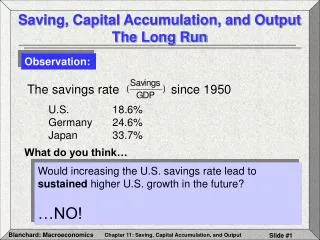
2. Saving and Growth Annual % change 1870-2000 Annual % change 1950-2000 Country 1870 1913 1950 1979 2000 Germany 1,205 2,320 5,005 18,014 23,247 2.3 3.1 Japan 963 1,825 2,216 16,899 24,772 2.5 4.8 United States 2,843 6,745 11,921 22,480 32,629 1.9 2.0 Since 1950 the US saving rate (S/Y) has averaged 18%. The German saving rate averaged 24% and the Japanese, 34%. Can this explain the growth differences? Probably not.

3. Preview • Suppose output rises. • A proportion of that, sY, is saved. • Assume S=I. Then I = sY. • Investment increases the capital stock. • With a greater capital stock, we can produce more. • Output rises.

4. Preview Capital Stock rises OutputRises OutputRises • Greater output leads to more saving, capital accumulation, and therefore more output. • Is this a perpetual cycle? • No. There are diminishing returns to capital. S and IRise

5. Preview Diminishing Returns Capital Accumulation A Fixed Proportion I = DK

6. Preview • There are diminishing returns to capital. • More capital will increase output, but at a decreasing rate. • Suppose population growth is positive. • Eventually, the increase in output won’t be enough to increase output-per-capita. • So there’s a “dynamic equilibrium”, a steady state of capital accumulation in the long run.

7. Interactions BetweenOutput and Capital 11-1 • Two important relations in the long run are: • The amount of capital determines the amount of output produced. • The amount of output determines the amount of saving and investment, and so the amount of capital accumulated.

8. The Effects of Capital on Output • The aggregate production function is a specification of the relation between aggregate output and the inputs in production. Y = aggregate output. K = capital — the sum of all the machines, plants, and office buildings in the economy. N = labor — the number of workers in the economy. The function F, tells us how much output is produced for given quantities of capital and labor.

9. The Effects of Capital on Output • Constant returns to scale implies that we can rewrite the aggregate production function as: • The amount of output per worker, Y/N depends on the amount of capital per worker, K/N. • As capital per worker increases, so does output per worker.

10. The Effects of Capital on Output • Under constant returns to scale, we can write the relation between output and capital per worker as follows: If we define Simplifying: More capital per worker produces more output per worker.

11. Output per Worker andCapital per Worker Output and Capital per Worker Increases in capital per worker lead to smaller and smaller increases in output per worker. An increase in capital per worker, K/N, causes a move along the production function.

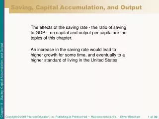
12. The Effects of Capital on Output • Focus on the role of capital accumulation: • The size of the population, the participation rate, and the unemployment rate are all constant. • Because this is the long run, it’s natural to assume that ut=ut-1. • This fit the concerns of the Classical economists: What determines the Wealth of Nations in the long run, when all prices are flexible?

13. The Effects of Capital on Output • Focus on the role of capital accumulation: • There is no technological progress. • Or, at least, we don’t know where it comes from. • Saving equals investment • Financial markets work perfectly.

14. The Effects of Capital on Output • Under these assumptions, the first important relation we want to express is between output and capital per worker: In words, higher capital per worker leads to higher output per worker.

15. The Effects of Output onCapital Accumulation Output and Investment: • The equations below describe the relation between private saving and investment:

16. The Effects of Output onCapital Accumulation • The saving rate (s) is the proportion of income that is saved (sY).

17. The Effects of Output onCapital Accumulation Output and Investment: • In the long run, private saving is equal to investment, and proportional to income. • Therefore, investment is proportional to output: • Higher output → higher saving→higher investment.

18. The Effects of Output onCapital Accumulation Investment and Capital Accumulation: • Suppose that capital is eternal (once installed, it’s there forever) • Then the evolution of the capital stock is given by: • Investment adds to capital.

19. The Effects of Output onCapital Accumulation Investment and Capital Accumulation: • More realistically, capital depreciates. • The evolution of the capital stock is given by: • Investment adds to capital. •  denotes the rate of depreciation. • A proportion (1- ) of capital remains from the previous period.

20. The Effects of Output onCapital Accumulation Investment and Capital Accumulation: • Combine the relation from output to investment, , and the relation from investment to capital accumulation, we get

21. The Effects of Output onCapital Accumulation Investment and Capital Accumulation: • If we divide this equation by N, we get

22. The Effects of Output onCapital Accumulation • Can we use this equation to know what will happen to capital per worker over time? Output and Capital per Worker:

23. The Effects of Output onCapital Accumulation • We can articulate the change in capital per worker over time by rearranging terms in the equation above. Output and Capital per Worker: In words, the change in the capital stock per worker (left side) is equal to saving per worker minus depreciation (right side).

24. The Effects of Output onCapital Accumulation Output and Capital per Worker: The stock of capital per worker will increase if The total amount of saving in the economy exceeds the part of the capital stock that is worn out.

25. Implications ofAlternative Saving Rates First relation:Capital determinesoutput. Second relation:Output determines capital accumulation 11-2 • Our two main relations are: • Combining the two relations, we can study the behavior of output and capital over time.

26. Dynamics of Capital and Output • From our main relations above, we express output per worker (Y/N) in terms of capital per worker to derive the equation below: change in capital from year t to year t+1 investment during year t depreciation during year t

27. Dynamics of Capital and Output change in capital from year t to year t+1 investment during year t depreciation during year t • If investment per worker (sY) exceeds depreciation per worker, the change in capital per worker is positive: Capital per worker increases. • If investment per worker is less than depreciation per worker, the change in capital per worker is negative: Capital per worker decreases.

28. Dynamics of Capital and Output Capital and Output Dynamics • Output per worker increases with capital per worker, but by less and less as capital per worker increases. • Investment per worker increases by a proportion of output per worker. • More capital per worker leads to more investment, but at a diminishing rate. • Suppose a country made a great effort to produce K/N and to save a bunch of output to invest it. The “extra bang for the extra buck” diminishes.

29. Dynamics of Capital and Output Capital and Output Dynamics When capital and output are low, investment exceeds depreciation, and capital increases. When capital and output are high, investment is less than depreciation and capital decreases. • At low levels of K/N, the “extra bang for the extra buck” invested is large, larger than what is being taken away by depreciation. • If the country already has a very large K/N, the “extra bang for the extra buck” invested is small and is overwhelmed by depreciation.

30. Dynamics of Capital and Output • At K0/N, capital per worker is low, investment exceeds depreciation, thus, capital per worker and output per worker tend to increase over time.

31. Dynamics of Capital and Output • At K*/N, output per worker and capital per worker remain constant at their long-run equilibrium levels.

32. Dynamics of Capital and Output • At K1/N, capital per worker is too high. Here investment is overwhelmed by depreciation. Therefore K/N and Y/N will fall over time. B C D A

33. Dynamics of Capital and Output • This model suggests convergence: • Take a poor country (one with low K/N) and a rich country (that has a high K/N). • The poor country will probably be farther away from K*/N than the rich country. • Then the poor country should grow faster than the rich country and catch up.

34. Dynamics of Capital and Output • This model suggests convergence: • Given the same level of technology and human capital, same institutions, etc., … • This model says that all countries should converge to the same level.

35. Dynamics of Capital and Output • This model suggests convergence: • High capital accumulation is not enough to sustain growth forever: if K/N is too high, diminishing returns will make investment to be lower than depreciation. • Compare Singapore with Hong Kong (case study).

36. Steady-State Capital and Output

37. Steady-State Capital and Output • The state in which output per worker and capital per worker are no longer changing is called the steady state of the economy. In steady state, the left side of the equation above equals zero, then: • The important point is to notice that there is one and only one value of K*/N that satisfies this equation.

38. Steady-State Capital and Output • There is only one value of K*/N that satisfies this equation: • Given the steady state of capital per worker (K*/N), the steady-state value of output per worker (Y*/N), is given by the production function: • There is only one steady-state value of Y*/N.

39. Steady-State Capital and Output • There is only one value of K*/N that satisfies this equation: • The steady-state values of K*/N and of Y*/N are uniquely determined by the saving rate. • A higher s will lead to a higher K*/N and a higher Y*/N. • But a higher s will leave the growth rate of Y*/N unaffected.

40. The Saving Rate and Output

41. The Saving Rate and Output • The effects of the saving rate on the growth rate of output per worker: • The saving rate has no effect on the long run growth rate of output per worker, which is equal to zero. • Output per worker and capital per worker are constant in the steady state. • If an economy wanted to increase the steady state K*/N every year it would have to increase savings/output every year.

42. The Saving Rate and Output • Nonetheless, the saving rate determines the level of output per worker in the long run. Other things equal, countries with a higher saving rate will achieve higher output per worker in the long run.

43. The Saving Rate and Output The Effects of Different Saving Rates A country that raises its saving rate achieves a higher level of output per worker in steady state. But, in the steady state, output/worker does not grow.

44. The Saving Rate and Output • Therefore, an increase in the saving rate will lead to higher growth of output per worker for some time, but not forever. • The saving rate does not affect the long-run growth rate of output per worker. • After an increase in the saving rate, growth will end once the economy reaches its new steady state.

45. The Saving Rate and Output The Effects of an Increase in the Saving Rate on Output per Worker An increase in the saving rate leads to a period of higher growth until output reaches its new higher steady-state level. The economy takes some time to reach the new steady state as it accumulates capital.

46. The Saving Rate and Output The Effects of an Increase in the Saving Rate on Output per Worker in an Economy with Technological Progress If there’s technological progress, the growth rate of Y/N is positive in the steady state. An increase in the saving rate leads to a period of higher growth until output reaches a new, higher path. (This is a logarithmic scale, so the slope of the steady-state path is equal to the growth rate of Y/N.)

47. The Optimal Saving Rate and Optimal Consumption

48. The Saving Rate and Consumption • The previous section suggests that a country could choose its steady state level of capital per worker and output per worker. • What steady state should a country choose? • I’d think that the steady state that maximizes consumption. • (Output is nice, but I’d focus on eating).

49. The Saving Rate and Consumption Steady statedepreciation / worker, dK*/N Steady state output / worker,f(K*/N) ? Steady stateoutput / worker, Y*/N Steady state investment / worker, sf(K*/N) Steady state capital / worker, K*/N

50. The Saving Rate and Consumption • Because people care about consumption (and not about investment or output), society should maximize steady-state consumption. Golden-rule saving rate Max consumption Golden-rule income Golden-rule level of capital/ worker