Download
1 / 68
790 likes | 1.53k Views
PART III Growth Theory: The Economy in the Very Long Run. Economic Growth I: Capital Accumulation and Population Growth. Chapter 8 of Macroeconomics , 8 th edition, by N. Gregory Mankiw ECO62 Udayan Roy. The Solow-Swan Model. This is a theory of macroeconomic dynamics

E N D
PART III Growth Theory: The Economy in the Very Long Run Economic Growth I: Capital Accumulation and Population Growth Chapter 8 of Macroeconomics, 8thedition, by N. Gregory Mankiw ECO62UdayanRoy
The Solow-Swan Model • This is a theory of macroeconomic dynamics • Using this theory, • you can predict where an economy will be tomorrow, the day after, and so on, if you know where it is today • you can predict the dynamic effects of changes in • the saving rate • the rate of population growth • and other factors
Two productive resources and one produced good • There are two productive resources: • Capital, K • Labor, L • These two productive resources are used to produce one • final good, Y
The Production Function • The production function is an equation that tells us how much of the final good is produced with specified amounts of capital and labor • Y = F(K, L) • Example: Y = 5K0.3L0.7
Constant returns to scale • Y = F(K, L) = 5K0.3L0.7 • Note: • if you double both K and L, Y will also double • if you triple both K and L, Y will also triple • … and so on • This feature of the Y = 5K0.3L0.7 production function is called constant returns to scale The Solow-Swan model assumes that production functions obey constant returns to scale
Constant returns to scale • Definition: The production function F(K, L) obeys constant returns to scale if and only if • for any positive number z (that is, z > 0) • F(zK, zL) = zF(K, L) • Example: Suppose F(K, L) = 5K0.3L0.7. • Then, for any z > 0, F(zK, zL) = 5(zK)0.3(zL)0.7 = 5z0.3K0.3z0.7L0.7 = 5z0.3 + 0.7K0.3L0.7 = z5K0.3L0.7 =zF(K, L) At this point, you should be able to do problem 1 (a) on page 232 of the textbook.
Constant returns to scale • CRS requires F(zK, zL) = zF(K, L) for any z > 0 • Let z be 1/L. • Then, So, y = F(k, 1) . From now on, F(k, 1) will be denoted f(k), the per worker production function. k = K/Ldenotes per worker stock of capital y = Y/Ldenotes per worker output So, y= f(k) .
Per worker production function: example At this point, you should be able to do problems 1 (b) and 3 (a) on pages 232 and 233 of the textbook. This is what a typical per worker production function looks like: concave
The Cobb-Douglas Production Function • Y = F(K, L) = 5K0.3L0.7 • This production function is itself an instance of a more general production function called the Cobb-Douglas Production Function • Y = AKαL1 − α , • where A is any positive number (A > 0) and • α is any positive fraction (1 > α > 0)
Per worker Cobb-Douglas production function • Y = AKαL1 − αimplies y = Akα = f(k) In problem 1 on page 232 of the textbook, you get Y = K1/2L1/2, which is the Cobb-Douglas production with A = 1 and α = ½. In problem 3 on page 233, you get Y = K0.3L0.7, which is the Cobb-Douglas production with A = 1 and α = 0.3.
Income, consumption, saving, investment • Output = income • The Solow-Swan model assumes that each individual saves a constant fraction, s, of his or her income • Therefore, saving per worker = sy = sf(k) • This saving becomes an addition to the existing capital stock • Consumption per worker is denoted c = y – sy = (1– s)y
Depreciation • But part of the existing capital stock wears out • This is called depreciation • The Solow-Swan model assumes that a constant fraction, δ, of the existing capital stock wears out in every period • That is, an individual who currently has k units of capital will lose δk units of capital though depreciation (or, wear and tear)
Depreciation • Although 0 < δ < 1 is the fraction of existing capital that wears out every period, in some cases—as in problem 1 (c) on page 219 of the textbook—depreciation is expressed as a percentage. • In such cases, care must be taken to convert the percentage value to a fraction • For example, if depreciation is given as 5 percent, you need to set δ = 5/100 = 0.05
Dynamics: what time is it? • We’ll attach a subscript to each variable to denote what date we’re talking about • For example, ktwill denote the economy’s per worker stock of capital on date tandkt+1 will denote the per worker stock of capital on date t + 1
How does per worker capital change? • A worker haskt units of capital on date t • He or she adds syt units of capital through saving • and loses δkt units of capital through depreciation • So, each worker accumulates kt + syt−δktunits of capital on date t + 1 • Does this mean kt+1 = kt + syt−δkt? • Not quite!
Population Growth • The Solow-Swan model assumes that each individual has n kids in each period • The kids become adult workers in the period immediately after they are born • and, like every other worker, have n kids of their own • and so on
Population Growth • Let the growth rate of any variable x be denoted xg. It is calculated as follows: • Therefore, the growth rate of the number of workers, Lg, is:
Dynamics: algebra Now we are ready for dynamics!
Dynamics: algebra At this point, you should be able to do problems 1 (d) and 3 (c) on pages 232 and 233 of the textbook. Please give them a try.
Dynamics: algebra to graphs Although this is the basic Solow-Swan dynamic equation, a simple modification will help us analyze the theory graphically. Now we are ready for graphical analysis.
Dynamics: algebra to graphs This version of the Solow-Swan equation will help us understand the model graphically.
Dynamics: algebra to graphs This version of the Solow-Swan equation will help us understand the model graphically. 2. The economy shrinks if and only if per worker saving and investment [sf(kt)] is less than (δ + n)kt. 3. The economy is at a steady state if and only if per worker saving and investment [sf(kt)] is equal to (δ + n)kt. 1. The economy grows if and only if per worker saving and investment [sf(kt)] exceeds (δ + n)kt. 4. (δ + n)kt is called break-even investment
Investment and break-even investment (δ + n)kt sf(kt) k1 k* Capital per worker, k Steady state
Investment and depreciation (δ + n)kt sf(kt) k1 investment Break-even investment k1 k* Capital per worker, k Moving toward the steady state Steady state
Investment and depreciation (δ + n)kt sf(kt) k1 k1 k* Capital per worker, k Moving toward the steady state k2 Steady state
Investment and depreciation (δ + n)kt sf(kt) k2 investment Break-even investment k1 k* Capital per worker, k Moving toward the steady state k2 Steady state
Investment and depreciation (δ + n)kt sf(kt) k2 k1 k* Capital per worker, k Moving toward the steady state k2 k3 Steady state
Investment and depreciation (δ + n)kt sf(kt) k1 k* Capital per worker, k Moving toward the steady state As long as k < k*, investment will exceed break-even investment, and k will continue to grow toward k* k2 k3 Steady state
The steady state: algebra • The economy eventually reaches the steady state • This happens when per worker saving and investment [sf(kt)] is equal to break-even investment [(δ + n)kt]. • For the Cobb-Douglas case, this condition is: At this point, you should be able to do problems 1 (c) and 3 (b) on pages 232 and 233 of the textbook. Please give them a try.
There is no growth! • The Solow-Swan model predicts that • Every economy will end up at the steady-state; in the long run, the growth rate is zero! • That is, k = k* and y = f(k*) = y* • Growth is possible—temporarily!—only if the economy’s per worker stock of capital is less than the steady state per worker stock of capital (k < k*) • If k < k*, the smaller the value of k, the faster the growth of k and y
From per worker to total • We have seen that per worker capital, k, is constant in the steady state • Now recall that k = K/L • and that L increases at the rate of n • Therefore,in the steady state, the total stock of capital, K, increases at the rate of n
From per worker to total • We have seen that per worker income y = f(k) is constant in the steady state • Now recall that y = Y/L • and that L increases at the rate of n • Therefore,in the steady state, the total income, Y, must also increase at the rate of n • Similarly,although per worker saving and investment, sy, is constant in the steady state, total saving and investment, sY, increases at the rate n
From per worker to per capita • Recall that L = amount of labor employed • Suppose P = amount of labor available • This is the labor force • But in the Solow-Swan model everybody is capable of work, even new-born children • So P can also be considered the population • Suppose u = fraction of population that is not engaged in production of the final good. • u is assumed constant • Then L = (1 – u)P or L/P= 1 – u
A sudden fall in capital per worker • A sudden decrease in k could be caused by: • Earthquake or war that destroys capital but not people • Immigration • A decrease in u • What does the Solow-Swan model say will be the result of this?
Investment and depreciation (δ + n)kt sf(kt) k1 k* Capital per worker, k A sudden fall in capital per worker At this point, you should be able to do problem 2 on pages 232 and 233 of the textbook. Please give it a try. 2. A gradual return to the steady state 1. A sudden decline