Download
1 / 22
220 likes | 336 Views
GRB Trigger Algorithms From DC1 to DC2. Nicola Omodei Riccardo Giannitrapani Francesco Longo Monica Brigida. DC1 Closeout status. Many people involved in GRB detection: I think that the generation of GRB has been a success! 4(+1) groups have been working on GRB detections: David Band

E N D
GRB Trigger AlgorithmsFrom DC1 to DC2 Nicola Omodei Riccardo Giannitrapani Francesco Longo Monica Brigida
DC1 Closeout status • Many people involved in GRB detection: I think that the generation of GRB has been a success! • 4(+1) groups have been working on GRB detections: • David Band • Jay Norris & Jerry Bonnell • Riccardo Giannitrapani et al. • Nicola Omodei • Tune Kamae et al.
Band’s method • Break up sky in instrument coordinates into regions, and apply rate triggers to each region. The regions are ~PSF in size (builds in knowledge of the instrument). • Use two (or more) staggered regions so that the burst will fall in the interior of a region. • Rate trigger—statistically significant increase in count rate averaged over time and energy bin.
Estimating the Background • The rate trigger requires an estimate of the background (=non-burst event rate). Typically the background is estimated from the non-burst lightcurve. • BUT here the event rate is so low that a region’s background estimated only from that region’s lightcurve will be dominated by Poisson noise. The event rate per region is a few×10-2 Hz. • Band’s current method is to average the background over the FOV, and apportion it to each region proportional to the effective area for that region.
Problem with Background Estimation • Problem: On short (~100 s) timescales the background is NOT uniform over the FOV. The ridge of emission along the Galactic plane causes many false triggers. • Solution (not implemented yet): Better model of the background. Region with false trigger • In the ~6 days of DC1 data,He found 16 bursts and 29 false triggers. • Note that his spatial grids extend to inclination angles of 65º and 70º. • The software He used was all home-grown IDL procedures.
Norris’s method • They used only one N-event sliding window as the first bootstrap step in searching for significant temporal-spatial clustering. Compute Log {Joint (spatial*temporal) likelihood} for tightest cluster in window: Log(P) = Log{ [1 – cos(di)] / 2 } + Log{ 1 – (1 + Xi) exp(-Xi) } • Their work is somewhat at 45 to main DC1 purposes. But DC1 set us up with all the equipment necessary to proceed: • Future emphasis will move to on-board recon problems: highest accuracy real-time triggers & localizations.
Very sensitive trigger — incorporates most of the useful information. • 17 detections: 11 on Day 1; 6 on Days 2-6. Some bright, some dim. • No false trigger.Formal expectation any detection is false << 10-6/day. • Additional aspects we will evaluate for on-board implementation: • Floating threshold; 2-D PSF; spatial clustering (Galactic Plane)
Riccardo’s method • The aim of the Riccardo talk was to present a analysis tool call “R” • He presented also an application of this tool for GRB searching, based on the quantile analysis. • He looks for outliers in the distribution of the count rate
Some improvements • Riccardo also compare the distribution of the counts with the Poisson distribution: The GRB are now really visible! Outliers
Some other improvements • Another way to see the outliers is looking at the (smoothed) counts map for (RA, TIME) coordinates (or for (DEC,TIME)); For all photons For outliers
Nicola’s method • First algorithm based on the trigger on the differential count rate (this get rid of the fluctuation of the background due to the galactic plane). • Very easy and fast algorithm!
The division of the sky • The same algorithm can be applied separately in sub region of the galactic map. This substantially reduces the background (non-burst events). 5 x 5 array reduces the “background” by a factor 25. Also faint burst can be detectable. Direct (70˚ x 36˚) information on the localization.
Comparing the results Generated 11 GRBs with spikes with more than 2 photons/second Burst photons GRB050718i Spectral analysis done with XSPEC (Monica) Light curves visualized Position in the sky map visualized
Common features and diversities • All of us triggered on the counts rate (in different ways): the gamma background (simulated) is low compared with the burst flux. • Both faint bursts (few tens of photons) and bright bursts (some hundreds of photons) have been successfully detected. • A big improvement of the burst trigger rate has been reached by dividing the sky map in smaller region. This procedure represents a big advantage in terms of background “reduction”. • David divide the sky map using instrument coordinates, maybe this is the reason of so many false triggers. • Nicola, Jay and Jerry used galactic coordinates: no false trigger. • Nicola developed a simple (and fast) algorithm and detect burst as much as Jay and Jerry did with more complicated algorithms. • Riccardo pointed out that one of the burst vanishes if the standard cuts are applied to the data. This means that with with a realistic background which requires a realistic background filter, some burst photons will be killed by the filter.
GRB Trigger, Alert & DC2 • On-board vs on-ground trigger algorithms. GBM comparison! • Develop a common interface for the burst alert algorithms • Better simulation of the background (including particles) • Background estimation • The development in other environments (IDL,Matlab,R, ROOT stand alone macros), is very useful, BUT the key point for the DC2 will be the development of science tools! SkyMap segmentation Background estimation On board On board recon (filter) Fast & Low memory consuming Buffer On ground Full recon High sensitivity No restriction on memory/time Trigger Algorithm Data storage Trigger on the counts rate Likelihood … Outliers
GRB Spectra EventBin + XSPEC (Francesco tutorial, XSPEC tutorial …..) Fitting models: power_law / grbm
GRB050720a 1634 counts Tstart: 176761 Tstop: 176880 Ra: 128 Dec: 65 Flux: 2.9 E-6 erg cm-2 s-1
Power law model Model: powerlaw<1> Model Fit Model Component Parameter Unit Value par par comp 1 1 1 powerlaw PhoIndex 1.74358 +/- 0.198269E-01 2 2 1 powerlaw norm 6.20041 +/- 1.32153 --------------------------------------------------------------------------- --------------------------------------------------------------------------- Chi-Squared = 849.3165 using 8 PHA bins. Reduced chi-squared = 141.5527 for 6 degrees of freedom Null hypothesis probability = 0.00
powerlaw • ignore **-1e5 1e8-** • Model: powerlaw<1> • Model Fit Model Component Param Unit Value • par par comp • 1 1 1 powerlaw PhoIndex 2.25854 +/- 0.403036E-01 • 2 1 powerlaw norm 12150.0 +/- 6275.72 • ----------------------------------------------------------------------- • ----------------------------------------------------------------------- • Chi-Squared = 36.43491 using 7 PHA bins. • Reduced chi-squared = 7.286983 for 5 degrees of freedom • Null hypothesis probability = 7.773E-07
GRB050718i 700 counts Tstart: 75415 Tstop: 75473 Ra: 92 Dec: 57 Flux: 2.6 E-6 erg cm-2 s-1 • GRB_050718i 75415 / 75474 ; 92 / 57 • Model: powerlaw<1> • Model Fit Model Component Parameter Unit Value • par par comp • 1 1 1 powerlaw PhoIndex 1.79878 +/- 0.280451E-01 • 2 2 1 powerlaw norm 18.8932 +/- 5.67197 • --------------------------------------------------------------------------- • --------------------------------------------------------------------------- • Chi-Squared = 212.8927 using 7 PHA bins. • Reduced chi-squared = 42.57854 for 5 degrees of freedom • Null hypothesis probability = 4.905E-44
GRB050718i powerlaw • ignore **-1e5 1e8-** • Model: powerlaw<1> • Model Fit Model Component Parameter Unit Value • par par comp • 1 1 1 powerlaw PhoIndex 2.16394 +/- 0.472441E-01 • 2 2 1 powerlaw norm 2908.87 +/- 1490.38 • --------------------------------------------------------------------------- • --------------------------------------------------------------------------- • Chi-Squared = 2.117105 using 7 PHA bins. • Reduced chi-squared = 0.4234209 for 5 degrees of freedom • Null hypothesis probability = 0.833