Download
1 / 33
330 likes | 421 Views
FT makes the New Yorker, October 4, 2010 page 71. The Fourier transform. regularity conditions Functions, A( ), - < < |A( )|d finite FT. a(t) = exp{it )A( )d - < < Inverse A( ) =(2 ) -1 exp{-i t} a(t) dt

E N D
The Fourier transform. regularity conditions Functions, A(), - < < |A()|d finite FT. a(t) = exp{it)A()d - < < Inverse A() =(2)-1 exp{-it} a(t) dt unique C()= A() + B() c(t) = c(t) + b(t) 2 1
Convolution (filtering). d(t) = b(t-s) c( s)ds D() = B()C() Discrete FT. a(t) = T-1 exp{i2ts/T} A(2s/T) s, t = 0,1,...,T-1 A(2s/T) = exp {-i2st/T) a(t) FFTs exist
Dirac delta. g() () d = g(0) exp {it}() d = 1 inverse () = (2)-1 exp {-it}dt Heavyside function H() = signum () () = dH()/d
Mixing. Stationary case unless otherwise indicated cov{dN(t+u),dN(t)} small for large |u| |pNN(u) - pNpN| small for large |u| hNN(u) = pNN(u)/pN ~ pN for large |u| qNN(u) = pNN(u) - pNpN u 0 |qNN(u)|du < cov{dN(t+u),dN(t)}= [(u)pN + qNN(u)]dtdu
Power spectral density. frequency-side, , vs. time-side, t /2 : frequency (cycles/unit time) fNN() = (2)-1 exp{-iu}cov{dN(t+u),dN(t)}/dt = (2)-1 exp{-iu}[(u)pN+qNN(u)]du = (2)-1pN + (2)-1 exp{-iu}qNN(u)]du Non-negative, symmetric Approach unifies analyses of processes of widely varying types
Filtering. dN(t)/dt = a(t-v)dM(v) = a(t-j ) = exp{it}A()dZM() with a(t) = (2)-1 exp{it}A()d dZN() = A() dZM() fNN() = |A()|2 fMM()
Association. Measuring? Due to chance? Are two processes associated? Eg. t.s. and p.p. How strongly? Can one predict one from the other? Some characteristics of dependence: E(XY) E(X) E(Y) E(Y|X) = g(X) X = g (), Y = h(), r.v. f (x,y) f (x) f(y) corr(X,Y) 0
Bivariate point process case. Two types of points (j ,k) Crossintensity. a rate Prob{dN(t)=1|dM(s)=1} =(pMN(t,s)/pM(s))dt Cross-covariance density. cov{dM(s),dN(t)} = qMN(s,t)dsdt no () often
Frequency domain approach. Coherency, coherence Cross-spectrum. Coherency. R MN() = f MN()/{f MM() f NN()} complex-valued, 0 if denominator 0 Coherence |R MN()|2 = |f MN()| 2 /{f MM() f NN()| |R MN()|2 1, c.p. multiple R2
Proof. Filtering. M = {j } a(t-v)dM(v) = a(t-j ) Consider dO(t) = dN(t) - a(t-v)dM(v)dt, (stationary increments) where A() = exp{-iu}a(u)du fOO () is a minimum at A() = fNM()fMM()-1 Minimum: (1 - |RMN()|2 )fNN() 0 |R MN()|2 1
Proof. Coherence, measure of the linear time invariant association of the components of a stationary bivariate process.
Regression analysis/system identification. dZN() = A() dZM() + error() A() = exp{-iu}a(u)du
Empirical examples. sea hare
Partial coherency. Trivariate process {M,N,O} “Removes” the linear time invariant effects of O from M and N
Time series variants. details later continuous time case Mixing. cov{Y(t+u),Y(t)} = cYY(u) small for large |u| |cYY(u)|du <
Power spectral density. frequency-side, , vs. time-side, t /2 : frequency (cycles/unit time) fYY() = (2)-1 exp{-iu}cov{Y(t+u),Y(t)} = (2)-1 exp{-iu}cYY(u)du -<< Non-negative, symmetric Approach unifies analyses of processes of widely varying types Things in the frequency domain look the same
Spectral representation. Y(t) = exp{it}dZY() - < t < ZY() random, complex-valued conj{ZY()} = ZY(-) E{dZY()} = ()cNd cov{dZY(),dZY()}=(-)f NN()dd cum{dZY(1),...,dZY(K)} = ...
Filtering. Yt) = a(t-v)X(v)dv = exp{it}A()dZX() with a(t) = (2)-1 exp{it}A()d dZY() = A() dZX() fYY() = |A()|2 fXX()
Bivariate time series case. (X(t),Y(t)) - < t < Cross-covariance function. general case cov{X(s),Y(t)} = cXY(s,t)
Spectral representation approach. FXY(.): cross-spectral measure
Frequency domain approach. Coherency, coherence Cross-spectrum. f XY()= (2)-1 exp{-iu)c XY(u)du -< < complex-valued Coherency. R XY() = f XY()/{f XX() f YY()} 0 if denominator 0 Coherence. |RXY()|2 = |f XY()| 2 /{fXX() fYY()| |RXY()|2 1, c.p. multiple R2
Regression analysis/system identification. dZY() = A() dZX() + error() A() = exp{-iu}a(u)du
Partial coherency. Trivariate process {X,Y,O} “Removes” the linear time invariant effects of O from X and Y