Download
1 / 35
360 likes | 505 Views
Image Segmentation. A Graph Theoretic Approach. Factors for Visual Grouping. Similarity (gray level difference) Proximity Continuity Reference: M. Wertheimer, “Laws of Organization in Perceptual Forms”, A Sourcebook of Gestalt Psychology, W.B. Ellis, ed., pp. 71-88, Harcourt, Brace, 1938.

E N D
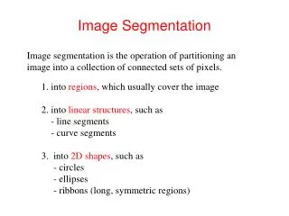
Image Segmentation A Graph Theoretic Approach
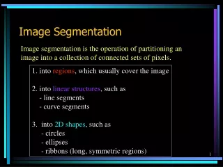
Factors for Visual Grouping • Similarity (gray level difference) • Proximity • Continuity Reference: M. Wertheimer, “Laws of Organization in Perceptual Forms”, A Sourcebook of Gestalt Psychology, W.B. Ellis, ed., pp. 71-88, Harcourt, Brace, 1938.
Subjectivity in Segmentation • Prior world knowledge needed • Agglomerative and divisive techniques in grouping (or Region-based merge and split algorithms in image segmentation) • Local properties – easier to specify but poorer results e.g. coherence of brightness, colour, texture, motion • Global properties – more difficult to specify but give better results e.g. object symmetries • Image segmentation can be modeled as a graph partitioning and optimization problem
Partitioning • Divisive or top-down approach • Inherently hierarchical • We must aim at returning a tree structure (called the dendogram) corresponding to a hierarchical partitioning scheme instead of a single “flat” partition
Challenges • Picking an appropriate criterion to minimize which would result in a “good” segmentation • Finding an efficient way to achieve the minimization
Modeling as a Graph Partitioning problem • Set of points of the feature space represented as a weighted, undirected graph, G = (V, E) • The points of the feature space are the nodes of the graph. • Edge between every pair of nodes. • Weight on each edge, w(i, j), is a function of the similarity between the nodes i and j. • Partition the set of vertices into disjoint sets where similarity within the sets is high and across the sets is low.
Weight Function for Brightness Images • Weight measure (reflects likelihood of two pixels belonging to the same object)
Segmentation and Graphs - Other Common Approaches • Minimal Spanning Tree • Limited Neighbourhood Set • Both approaches are computationally efficient but the criteria are based on local properties • Perceptual grouping is about extracting global impressions of a scene; thus local criteria are often inadequate
First attempt at global criterion selection • A graph can be partitioned into two disjoint sets by simply removing the edges connecting the two parts • The degree of dissimilarity between these two pieces can be computed as total weight of the edges that have been removed • More formally, it is called the ‘cut’
Optimization Problem • Minimize the cut value • No of such partitions is exponential (2^N) but the minimum cut can be found efficiently Reference: Z. Wu and R. Leahy, “An Optimal Graph Theoretic Approach to Data Clustering: Theory and Its Application to Image Segmentation”. IEEE Trans. Pattern Analysis and Machine Intelligence, vol. 15, no. 11, pp. 1101-1113, Nov. 1993. Subject to the constraints:
Problems with min-cut • Minimum cut criteria favors cutting small sets of isolated nodes in the graph.
Solution – Normalized Cut • We must avoid unnatural bias for partitioning out small sets of points • Normalized Cut - computes the cut cost as a fraction of the total edge connections to all the nodes in the graph where
Looking at it another way.. • Our criteria can also aim to tighten similarity within the groups • Minimizing Ncut and maximizing Nassoc are actually equivalent
Matrix Formulations Let x be an indicator vector s.t. xi = 1, if i belongs to A 0, otherwise • Assoc(A, A) = xTWx • Assoc(A, V) = xTDx • Cut(A, V-A) = xT(D – W)x
Computational Issues • Exact solution to minimizing normalized cut is an NP-complete problem • However, approximate discrete solutions can be found efficiently • Normalized cut criterion can be computed efficiently by solving a generalized eigenvalue problem
Algorithm 1. Construct the weighted graph representing the image. Summarize the information into matrices, W & D. Edge weight is an exponential function of feature similarity as well as distance measure. 2. Solve for the eigenvectors with the smallest eigenvalues of: (D – W)x = LDx
Algorithm (contd.) 3. Partition the graph into two pieces using the second smallest eigenvector. Signs tell us exactly how to partition the graph. 4. Recursively run the algorithm on the two partitioned parts. Recursion stops once the Ncut value exceeds a certain limit. This maximum allowed Ncut value controls the number of groups segmented.
Computational Issues Revisited • Solving a standard eigenvalue problem for all eigenvectors takes O(n^3) operations, where n is the number of nodes in the graph • This becomes impractical for image segmentation applications where n is the number of pixels in an image • For the problem at hand, the graphs are often only locally connected, only the top few eigenvectors are needed for graph partitioning, and the precision requirement for the eigenvectors is low, often only the right sign bit is required.
A Physical Interpretation • Think of the weighted graph as a spring mass system • Graph nodes physical masses • Graph edges springs • Graph edge weight spring stiffness • Total incoming edge weights mass of the node
A Physical Interpretation (contd..) • Imagine giving a hard shake to this spring-mass system, forcing the nodes to oscillate in the direction perpendicular to the image plane • Nodes that have stronger spring connections among them will likely oscillate together • Eventually, the group will “pop” off from the image plane • The overall steady state behavior of the nodes can be described by its fundamental mode of oscillation and it can be shown that the fundamental modes of oscillation of this spring mass system are exactly the generalized eigenvectors of the normalized cut.
Comparisons with other criteria • Average Cut: • Analogously, Average Association can be defined as: • Unlike in the case of Normalized Cut and Normalized Association, Average Cut and Average Association do not have a simple relationship between them • Consequently, one cannot simultaneously minimize the disassociation across the partitions while maximizing the association within the groups • Normalized Cut produces better results in practice
Comparisons with other criteria (contd..) • Average association has a bias for finding tight clusters – runs the risk of finding small, tight clusters in the data • Average cut does not look at within-group similarity – problems when the dissimilarity between groups is not clearly defined
Consider random 1-D data points: • Each data point is a node in the graph and the weighted graph edge connecting two points is defined to be inversely proportional to the distance between two nodes • We will consider two different monotonically decreasing weight functions, w(i,j) = f(d(i,j)), defined on the distance function, d(i,j), with differents rate of fall-off.
Fast falling weight function • With this function, only close-by points are connected.
Criterion used Second smallest eigenvector plot
Interpretation The cluster on the right has less within-group similarity compared with the cluster on the left. In this case, average association fails to find the right partition. Instead, it focuses on finding small clusters in each of the two main subgroups.
Slowly decreasing weight function • With this function, most points have non-trivial connections with the rest
Criterion used Second smallest eigenvector plot
Interpretation To find a cut of the graph, a number of edges with heavy weights have to be removed. In this case, average cut has trouble deciding on where to cut.
Reference J. Shi and J. Malik, “Normalized Cuts and Image Segmentation,” IEEE Trans. Pattern Analysis and Machine Intelligence, vol. 22, no. 8, pp. 888-905, Aug. 2000.