Download
1 / 14
140 likes | 333 Views
6 - 2. Basic Statistics. A statistic is a number, computed from sample data, such as a mean or variance.The objective of Statistics is to make inferences (predictions, decisions) about a population based upon information contained in a sample.MendenhallThe objective of Statistics is to make predictions about the cost of a weapon system based upon information in analogous systems.DoD Cost Analyst.

E N D
1. 6 - 1 Basic Univariate Statistics Chapter 6
2. 6 - 2
3. 6 - 3 Measures of Central Tendency These statistics describe the �middle region� of the sample.
Mean
The arithmetic average of the data set.
Median
The �middle� of the data set.
Mode
The value in the data set that occurs most frequently.
These are almost never the same, unless you have a perfectly symmetric, unimodal population.
4. 6 - 4 Mean The Sample Mean ( ) is the arithmetic average of a data set.
It is used to estimate the population mean, (m).
Calculated by taking the sum of the observed values (yi) divided by the number of observations (n).
5. 6 - 5 Median The Median is the middle observation of an ordered (from low to high) data set
Examples:
1, 2, 4, 5, 5, 6, 8
Here, the middle observation is 5, so the median is 5
1, 3, 4, 4, 5, 7, 8, 8
Here, there is no �middle� observation so we take the average of the two observations at the center
6. 6 - 6 Mode The Mode is the value of the data set that occurs most frequently
Example:
1, 2, 4, 5, 5, 6, 8
Here the Mode is 5, since 5 occurred twice and no other value occurred more than once
Data sets can have more than one mode, while the mean and median have one unique value
Data sets can also have NO mode, for example:
1, 3, 5, 6, 7, 8, 9
Here, no value occurs more frequently than any other, therefore no mode exists
You could also argue that this data set contains 7 modes since each value occurs as frequently as every other
7. 6 - 7 Dispersion Statistics The Mean, Median and Mode by themselves are not sufficient descriptors of a data set
Example:
Data Set 1: 48, 49, 50, 51, 52
Data Set 2: 5, 15, 50, 80, 100
Note that the Mean and Median for both data sets are identical, but the data sets are glaringly different!
The difference is in the dispersion of the data points
Dispersion Statistics we will discuss are:
Range
Variance
Standard Deviation
8. 6 - 8 Range The Range is simply the difference between the smallest and largest observation in a data set
Example
Data Set 1: 48, 49, 50, 51, 52
Data Set 2: 5, 15, 50, 80, 100
The Range of data set 1 is 52 - 48 = 4
The Range of data set 2 is 100 - 5 = 95
So, while both data sets have the same mean and median, the dispersion of the data, as depicted by the range, is much smaller in data set 1
9. 6 - 9 Variance The Variance, s2, represents the amount of variability of the data relative to their mean
As shown below, the variance is the �average� of the squared deviations of the observations about their mean
10. 6 - 10 Standard Deviation The Variance is not a �common sense� statistic because it describes the data in terms of squared units
The Standard Deviation, s, is simply the square root of the variance
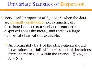
11. 6 - 11 Standard Deviation The sample standard deviation, s, is measured in the same units as the data from which the standard deviation is being calculated
12. 6 - 12 Coefficient of Variation For a given data set, the standard deviation is $100,000.
Is that good or bad? It depends�
A standard deviation of $100K for a task estimated at $5M would be very good indeed.
A standard deviation of $100K for a task estimated at $100K is clearly useless.
What constitutes a �good� standard deviation?
The �goodness� of the standard deviation is not its value per se, but rather what percentage the standard deviation is of the estimated value.
The Coefficient of Variation (CV) is defined as the �average� percent estimating error when predicting subsequent observations within the representative population.
The CV is the ratio of the standard deviation to the mean.
13. 6 - 13 Coefficient of Variation In the first example, the CV is $100K/$5M = 2%
In the second example, the CV is $100K/$100K = 100%
These values are unitless and can be readily compared.
The CV is the �average� percent estimating error for the population when using as the estimator.
Or, the CV is the �average� percent estimating error when estimating the cost of future tasks.
Calculate the CV from our previous transmogrifier cost database:
CV = $6.67K/$9.06K = 73.6%
Therefore, for subsequent observations we would expect to be off on �average� by 73.6% when using $9.06K as the estimated cost.
14. 6 - 14 Normal Distribution