Download

1 / 23
1.1k likes | 2.35k Views
Introduction to COMSOL. Travis Campbell Developed for CHE 331 – Fall 2012 Oregon State University School of Chemical, Biological and Environmental Engineering. What is COMSOL?. C ourse requirement Modeling and simulation software Tool for system design/optimization

E N D
Introduction to COMSOL Travis Campbell Developed for CHE 331 – Fall 2012 Oregon State University School of Chemical, Biological and Environmental Engineering
What is COMSOL? • Course requirement • Modeling and simulation software • Tool for system design/optimization • Method for checking work
A Brief History of Modeling Software • “A computer model refers to the algorithms and equations used to capture the behavior of the system being modeled. However, a computer simulation refers to the actual running of the program which contains these equations or algorithms.”1 http://en.wikipedia.org/wiki/Computer_model • Developed rapidly with computers • Influencing research
The General Idea Behind Numerical Modeling • User builds a model with significant variables • User builds a model mesh • COMSOL solves the model numerically at every mesh intersection • Intersections are connected to provide “continuous” data
How is the model solved at every intersection? • Several methods exist - one example is the Finite Element Method: ) +
COMSOL Step by Step for 4 Models • Model 1 – Laminar Flow in a Pipe • Model 2 – Turbulent Flow in a Pipe • Model 3 – Laminar Flow between Parallel Plates • Model 4 – Flow of a Falling Film • These notes apply to Version 4.2, only!
COMSOL Model 1 – Laminar Flow in a Pipe • Open COMSOL • Select Space Dimension 2D, click • Add Physics Laminar Flow, click • Select Study Type Stationary, click • In Main Menu, select View > Desktop Layout > Reset Desktop MAIN MENU MODEL BUILDER MENU MODEL SUB MENU GRAPHICS
COMSOL Model 1 – Laminar Flow in a Pipe • In Model Builder Menu, right-click Geometry 1 and select Rectangle • Select Rectangle 1 • In Model Sub Menu, enter Width: 5 m, Height: 0.1 m • Click Build Selected • In Model Builder Menu, right-click Materialsand select Open Material Browser • In Model Sub Menu, select Liquids and Gases> Liquids > Water • Click Add Material to Model (click twice) • In Model Builder Menu, click Laminar Flow • In Model Sub Menu, select Physical Model>Compressibility> Incompressible flow • In Model Builder Menu, right-click Laminar Flow and select Inlet • Select Inlet 1
COMSOL Model 1 – Laminar Flow in a Pipe • Define first Boundary Condition by describing the inlet velocity (average velocity).On the Graphic, select the left boundary • In Model Sub Menu, click Add to Selection • In Model Sub Menu, select Boundary Condition > Velocity. Click Normal Inflow Velocity. Enter Uo = 0.001 m/s. • In Model Builder Menu, right click Laminar Flow and select Outlet • Select Outlet 1 • Define second Boundary Condition by describing the outlet pressure. On the Graphic, select the right boundary • In Model Sub Menu, click Add to Selection • In Model Sub Menu, select Boundary Condition >Pressure, no viscous stress. Enter po= 0 Pa.
COMSOL Model 1 – Laminar Flow in a Pipe • Add no slip conditions at the pipe walls. In Model Builder Menu, click Laminar Flow > Wall 1 • In Model Sub Menu, confirm that Boundaries 2, 3 only are selected • In Model Sub Menu, select Boundary Condition > No slip • In Model Builder Menu, click Mesh • Select Physics-controlled mesh, Normal Element size • In Model Builder Menu, right-click Study 1and select Compute to simulate your model. Note the Reynolds number:
COMSOL Model 1 – Laminar Flow in a Pipe Time required to run your simulation depends on many factors: • Processor speed • Connection speed • Model size • Mesh granularity Results can be analyzed in many ways. We will find the velocity profile as a function of pipe cross-section.
COMSOL Model 1 – Laminar Flow in a Pipe • In Model Builder Menu, expand Results. Right-click Data Setsand select Cut Line 2D. • Select Cut Line 2D 1 • In Model Sub Menu, select Data set>Solution 1 and enter Line Data: • Click Plot • In Model Builder Menu, right-click Results and select 1D Plot Group • Select 1D Plot Group 1 • In Model Sub Menu, select Data > Data set > Cut Line 2D 1 • In Model Builder Menu, right-click 1D Plot Group 1and select Line Graph • Select Line Graph 1 • In Model Sub Menu, select Data >Data set >From parent • Confirm that the y-Axis Data is velocity, spf.U [m/s] • Click Plot
COMSOL Step by Step Models to be completed • Model 1 – Laminar Flow in a Pipe • Model 2 – Turbulent Flow in a Pipe • Model 3 – Laminar Flow between Parallel Plates • Model 4 – Flow of a Falling Film
COMSOL Model 2 - Turbulent Flow in a Pipe • Similar to Laminar Flow in a Pipe • Differences: • 3. Turbulent Flow (k-ε) • 19. Enter Uo = 10 m/s • 27. In Model Sub Menu, select Boundary Condition >Wall Functions • Re = 1e6
COMSOL Step by Step Models to be completed • Model 1 – Laminar Flow in a Pipe • Model 2 – Turbulent Flow in a Pipe • Model 3 – Laminar Flow between Parallel Plates • Model 4 – Flow of a Falling Film
COMSOL Model 3 – Laminar Flow between Parallel Plates • Also similar to Laminar Flow in a Pipe • Differences: • 19. In Model Sub Menu, select Boundary Condition > Pressure, no viscous stress. Enter po = 0 Pa. Note that both Inlet and Outlet Boundary Conditions are zero pressure. What does this mean? • After 19: • In Model Builder Menu, right click Laminar Flow and select Wall • Select Wall 2 • Define third Boundary Condition by describing the upper plate velocity. On the Graphic, select the top boundary • In Model Sub Menu, click Add to Selection • In Model Sub Menu, select Boundary Condition >Moving Wall. Enter uw= (0.001, 0) Pa. • 26. In Model Sub Menu, confirm that Boundary 2 only is selected
COMSOL Step by Step Models to be completed • Model 1 – Laminar Flow in a Pipe • Model 2 – Turbulent Flow in a Pipe • Model 3 – Laminar Flow between Parallel Plates • Model 4 – Flow of a Falling Film
COMSOL Model 4 – Flow of a Falling Film • Most similar to Laminar Flow between Parallel Plates • Differences: • Make rectangle tall and skinny (W: 0.001 m, H: 0.05 m) • Boundary conditions: • Wall 1 – No Slip • Wall 2 – Outlet, zero pressure • Wall 3 – Inlet, zero velocity • Wall 4 – Open boundary, zero normal stress • Add Volume Force to Laminar Flow with -9810 N/m3 in the y-direction • Make a horizontal cut line near the bottom of your geometry, to capture the “fully developed” film flow