Download
1 / 15
160 likes | 436 Views
Modeling Ocean Currents in COMSOL. Reza Malek-Madani Kevin McIlhany U. S. Naval Academy 24 Oct, 2006 rmm@usna.edu. CCBOM. Center for Chesapeake Bay Observation and Modeling Mathematics Oceanography Physics Ocean Engineering Chemistry. Acoustic Wave and Current Profiler (AWAC).

E N D
Modeling Ocean Currents in COMSOL Reza Malek-Madani Kevin McIlhany U. S. Naval Academy 24 Oct, 2006 rmm@usna.edu
CCBOM • Center for Chesapeake Bay Observation and Modeling • Mathematics • Oceanography • Physics • Ocean Engineering • Chemistry Acoustic Wave and Current Profiler (AWAC)
Velocity Vector Field, Chesapeake Bay, Dec 27, 1999, Courtesy of Tom Gross, NOAA, Coastal Survey Division http://chartmaker.ncd.noaa.gov/csdl/op/images/UVanim.gif
dx/dt = u(x, y, z, t), dy/dt = v(x, y, z, t)
How do the errors in the velocity field affect the errors in the dynamical systems computations and the particle fates? • Are the statistics of the particle trajectories stable and realizable relative to the statistics of the velocity field? • Are stable and unstable manifolds of the system dx/dt = u, dy/dt = v computable if u and v are known only locally in time (90 day date length) and in space (incomplete data collection)? • New hydrodynamic model
Goals and Strategy • Goals: • Obtain velocity field for the dynamics of the Chesapeake Bay, based on real wind and planetary forcing, and • Apply dynamical systems tools to the velocity field to understand transport and mixing in the Bay. • Strategy: First consider reduced models. • Qualitative Models: Simple geometry – Emphasis on PDEs - Stommel, Munk, Veronis, 2 1/2 layer model, Navier-Stokes, nonlinear Ellipitic PDEs • Complex Geometries: 2D and 3D boundaries of the Chesapeake Bay. Eigenvalue and Poisson Solvers • Comparison With Quoddy (NOAA) model
Stommel’s model 1948 paper, Key Assumptions: 2D, Steady, Rectangular Basin, Bottom Friction Key Features: Wind stress, Coriolis Key Findings: Boundary Layer (“Gulf Stream”) • = stream function Boundary conditions: = 0 on all four boundaries Scales: N. Atlantic Basin: 10,000 Km by 6000 Km Depth: 200 Meters Coriolis Parameter: 10^(-13)
Munk’s Model Zero boundary conditions Multiphysics approach