Download
1 / 64
650 likes | 768 Views
Chapter 12. Monopolistic Competition and Oligopoly. Monopolistic Competition. Characteristics Many firms Free entry and exit Differentiated product. Monopolistic Competition. The amount of monopoly power depends on the degree of differentiation

E N D
Chapter 12 Monopolistic Competition and Oligopoly
Monopolistic Competition • Characteristics • Many firms • Free entry and exit • Differentiated product Chapter 12
Monopolistic Competition • The amount of monopoly power depends on the degree of differentiation • Examples of this very common market structure include: • Toothpaste • Soap • Cold remedies • Retail Chapter 12
Monopolistic Competition • Two important characteristics • Differentiated but highly substitutable products (cross-price elasticity of demand large) • Free entry and exit (keeps profits down) Chapter 12
MC MC AC AC PSR PLR DSR DLR MRSR MRLR QSR QLR A Monopolistically CompetitiveFirm in the Short and Long Run $/Q $/Q Short Run Long Run Quantity Quantity
A Monopolistically CompetitiveFirm in the Short and Long Run • Short run • Downward sloping demand – differentiated product • Demand is relatively elastic – good substitutes • MR < P • Profits are maximized when MR = MC • This firm is making economic profits Chapter 12
A Monopolistically CompetitiveFirm in the Short and Long Run • Long run • Profits will attract new firms to the industry (no barriers to entry) • The old firm’s demand will decrease to DLR • Firm’s output and price will fall • Industry output will rise • No economic profit (P = AC) • P > MC some monopoly power Chapter 12
Deadweight loss MC AC MC AC P PC D = MR DLR MRLR QC QMC Monopolistically and Perfectly Competitive Equilibrium (LR) Monopolistic Competition Perfect Competition $/Q $/Q Quantity Quantity
Monopolistic Competition and Economic Efficiency • The monopoly power yields a higher price than perfect competition. If price was lowered to the point where MC = D, consumer surplus would increase by the yellow triangle – deadweight loss. • With no economic profits in the long run, the firm is still not producing at minimum AC and excess capacity exists. Chapter 12
Monopolistic Competition and Economic Efficiency • Firm faces downward sloping demand so zero profit point is to the left of minimum average cost • Excess capacity is inefficient because average cost would be lower with fewer firms Chapter 12
Excess Capacity • The FIRM’s output is inefficiently low: less than minimum ATC • Fewer total firms in the INDUSTRY would increase the FIRM’s demand and allow them to take advantage of economies of scale and increase output Chapter 12
Monopolistic Competition • If inefficiency is bad for consumers, should monopolistic competition be regulated? • Market power is relatively small. Usually there are enough firms to compete with enough substitutability between firms – deadweight loss small. • Inefficiency is balanced by benefit of increased product diversity – may easily outweigh deadweight loss. Chapter 12
Oligopoly – Characteristics • Small number of firms • Product differentiation may or may not exist • Barriers to entry • Scale economies • Patents • Technology access ($$) • Name recognition ($$) • Strategic action Chapter 12
Oligopoly • Examples • Automobiles • Steel • Aluminum • Petrochemicals • Electrical equipment Chapter 12
Oligopoly • Management Challenges • Strategic actions to deter entry • Threaten to decrease price against new competitors by keeping excess capacity • Rival behavior • Because only a few firms, each must consider how its actions will affect its rivals and in turn how their rivals will react Chapter 12
Oligopoly – Equilibrium • If one firm decides to cut their price, they must consider what the other firms in the industry will do • Could cut price some, the same amount, or more than firm • Could lead to price war and drastic fall in profits for all • Actions and reactions are dynamic, evolving over time Chapter 12
Oligopoly – Equilibrium • Defining Equilibrium • Firms are doing the best they can and have no incentive to change their output or price • All firms assume competitors are taking rival decisions into account • Nash Equilibrium • Each firm is doing the best it can given what its competitors are doing • We will focus on duopoly • Markets in which two firms compete Chapter 12
Oligopoly • The Cournot Model • Oligopoly model in which firms produce a homogeneous good, each firm treats the output of its competitors as fixed, and all firms decide simultaneously how much to produce • Market price depends on the total output of both firms • Firm will adjust its output based on what it thinks the other firm will produce Chapter 12
Firm 1 and market demand curve, D1(0), if Firm 2 produces nothing. D1(0) If Firm 1 thinks Firm 2 will produce 50 units, its demand curve is shifted to the left by this amount. If Firm 1 thinks Firm 2 will produce 75 units, its demand curve is shifted to the left by this amount. MR1(0) D1(75) MR1(75) MC1 MR1(50) D1(50) 12.5 25 50 Firm 1’s Output Decision P1 Q1 Chapter 12
Oligopoly • The Reaction Curve • The relationship between a firm’s profit-maximizing output and the amount it thinks its competitor will produce • A firm’s profit-maximizing output is a decreasing schedule of the expected output of Firm 2 • Different MC = different reaction functions Chapter 12
Firm 2’s Reaction Curve Q*2(Q1) Firm 1’s Reaction Curve Q*1(Q2) Reaction Curves and Cournot Equilibrium Q1 Firm 1’s reaction curve shows how much it will produce as a function of how much it thinks Firm 2 will produce. The x’s correspond to the previous model. 100 75 Firm 2’s reaction curve shows how much it will produce as a function of how much it thinks Firm 1 will produce. 50 x x 25 x x Q2 25 50 75 100 Chapter 12
Firm 2’s Reaction Curve Q*2(Q1) Cournot Equilibrium Firm 1’s Reaction Curve Q*1(Q2) Reaction Curves and Cournot Equilibrium Q1 100 In Cournot equilibrium, each firm correctly assumes how much its competitors will produce and thereby maximizes its own profits. 75 50 x x 25 x x Q2 25 50 75 100 Chapter 12
Cournot Equilibrium • Each firm’s reaction curve tells it how much to produce given the output of its competitor • Equilibrium in the Cournot model, in which each firm correctly assumes how much its competitor will produce and sets its own production level accordingly Chapter 12
Oligopoly • Cournot equilibrium is an example of a Nash equilibrium (Cournot-Nash Equilibrium) • The Cournot equilibrium says nothing about the dynamics of the adjustment process • Since both firms adjust their output, neither output would be fixed Chapter 12
The Linear Demand Curve • An Example of the Cournot Equilibrium • Two firms face linear market demand curve • We can compare competitive equilibrium, the equilibrium resulting from collusion, and Cournot Equilibrium • Market demand is P = 30 - Q • Q is total production of both firms: Q = Q1 + Q2 • Both firms have MC1 = MC2 = 0 Chapter 12
Oligopoly Example: Cournot • Firm 1’s Reaction Curve MR = MC Chapter 12
Oligopoly Example • An Example of the Cournot Equilibrium Chapter 12
Oligopoly Example • An Example of the Cournot Equilibrium Chapter 12
30 Firm 2’s Reaction Curve Cournot Equilibrium 15 10 Firm 1’s Reaction Curve 10 15 30 Duopoly Example Q1 The demand curve is P = 30 - Q and both firms have 0 marginal cost. Q2 Chapter 12
Oligopoly Example • Profit Maximization with Collusion • Collusion implies industry profits maximized Chapter 12
Profit Maximization w/ Collusion • Contract Curve • Q1 + Q2 = 15 • Shows all pairs of output Q1 and Q2 that maximize total profits • Q1 = Q2 = 7.5 • Less output and higher profits than the Cournot equilibrium Chapter 12
Firm 2’s Reaction Curve Competitive Equilibrium (P = MC; Profit = 0) 15 Cournot Equilibrium Collusive Equilibrium 10 7.5 Firm 1’s Reaction Curve Collusion Curve 7.5 10 15 Duopoly Example Q1 For the firm, collusion is the best outcome followed by the Cournot Equilibrium and then the competitive equilibrium 30 Q2 30 Chapter 12
Review: How to solve Cournot • Begin with Total Revenue function • Create by calculating P times Q1 and P is from the demand function in terms of Q total • Must substitute Q1 + Q2 for Q • Result: TR function in terms of Q1 and Q2 • Identify Marginal Revenue and set equal to Marginal Cost • Solve this equality in terms of Q1 = fn. Of Q2 Chapter 12
First Mover Advantage – The Stackelberg Model • Oligopoly model in which one firm sets its output before other firms do • Assumptions • One firm can set output first • MC = 0 • Market demand is P = 30 - Q where Q is total output • Firm 1 sets output first and Firm 2 then makes an output decision seeing Firm 1’s output Chapter 12
First Mover Advantage – The Stackelberg Model • Firm 1 • Must consider the reaction of Firm 2 • Firm 2 • Takes Firm 1’s output as fixed and therefore determines output with the Cournot reaction curve: Q2 = 15 - ½(Q1) Chapter 12
First Mover Advantage – The Stackelberg Model • Firm 1 • Choose Q1 so that: • Firm 1 knows Firm 2 will choose output based on its reaction curve. We can use Firm 2’s reaction curve as Q2 . Chapter 12
First Mover Advantage – The Stackelberg Model • Using Firm 2’s Reaction Curve for Q2: Chapter 12
First Mover Advantage – The Stackelberg Model • Conclusion • Going first gives Firm 1 the advantage • Firm 1’s output is twice as large as Firm 2’s • Firm 1’s profit is twice as large as Firm 2’s • Going first allows Firm 1 to produce a large quantity. Firm 2 must take that into account and produce less unless it wants to reduce profits for everyone. Chapter 12
Price Competition • Competition in an oligopolistic industry may occur with price instead of output • The Bertrand Model is used • Oligopoly model in which firms produce a homogeneous good, each firm treats the price of its competitors as fixed, and all firms decide simultaneously what price to charge Chapter 12
Price Competition – Bertrand Model • Assumptions • Homogenous good • Market demand is P = 30 - Q where Q = Q1 + Q2 • MC1 = MC2 = $3 • Can show the Cournot equilibrium if Q1 = Q2 = 9 and market price is $12, giving each firm a profit of $81. Chapter 12
Price Competition – Bertrand Model • Assume here that the firms compete with price, not quantity • Since good is homogeneous, consumers will buy from lowest price seller • If firms charge different prices, consumers buy from lowest priced firm only • If firms charge same price, consumers are indifferent who they buy from and each firm will supply half the market Chapter 12
Price Competition – Bertrand Model • Nash equilibrium is competitive equilibrium output since have incentive to cut prices • Both firms set price equal to MC • P = MC; P1 = P2 = $3 • Q = 27; Q1 & Q2 = 13.5 • Both firms earn zero profit Chapter 12
Price Competition – Bertrand Model • Why not charge a different price? • If charge more, sell nothing • If charge less, lose money on each unit sold • The Bertrand model demonstrates the importance of the strategic variable • Price versus output Chapter 12
Bertrand Model – Criticisms • When firms produce a homogenous good, it is more natural to compete by setting quantities rather than prices • Even if the firms do choose the same price, what share of total sales will go to each one? • Probably not exactly half Chapter 12
Competition Versus Collusion:The Prisoners’ Dilemma • Nash equilibrium is a noncooperative equilibrium: each firm makes decision that gives greatest profit, given actions of competitors • Although collusion is illegal, why don’t firms cooperate without explicitly colluding? • Why not set profit maximizing collusion price and hope others follow? Chapter 12
Competition Versus Collusion:The Prisoners’ Dilemma • Competitor is not likely to follow • Competitor can do better by choosing a lower price, even if they know you will set the collusive level price • We can use a payoff matrix to better understand the firms’ choices Chapter 12
$12, $12 $20, $4 $4, $20 $16, $16 Payoff Matrix for Pricing Game Firm 2 Charge $4 Charge $6 Charge $4 Firm 1 Charge $6 Chapter 12
Competition Versus Collusion:The Prisoners’ Dilemma • We can now answer the question of why firm does not choose cooperative price • Cooperating means both firms charging $6 instead of $4 and earning $16 instead of $12 • Each firm always makes more money by charging $4, no matter what its competitor does • Unless enforceable agreement to charge $6, will be better off charging $4 Chapter 12
Competition Versus Collusion:The Prisoners’ Dilemma • An example in game theory, called the Prisoners’ Dilemma, illustrates the problem oligopolistic firms face • Two prisoners have been accused of collaborating in a crime • They are in separate jail cells and cannot communicate • Each has been asked to confess to the crime Chapter 12
-5, -5 -1, -10 -10, -1 -2, -2 Payoff Matrix for Prisoners’ Dilemma Prisoner B Confess Don’t confess Confess Prisoner A Would you choose to confess? Don’t confess Chapter 12