Inference in first-order logic

1. Inference in first-order logic

2. Outline • Reducing first-order inference to propositional inference • Unification • Generalized Modus Ponens • Forward chaining • Backward chaining • Resolution

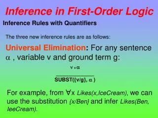
3. Universal instantiation (UI) • Every instantiation of a universally quantified sentence is entailed by it: vαSubst({v/g}, α) for any variable v and ground term g • E.g., x King(x) Greedy(x)  Evil(x) yields: King(John) Greedy(John) Evil(John) King(Richard) Greedy(Richard) Evil(Richard) King(Father(John)) Greedy(Father(John)) Evil(Father(John)) . . .

4. Existential instantiation (EI) • For any sentence α, variable v, and constant symbol k that does not appear elsewhere in the knowledge base: vα Subst({v/k}, α) • E.g., xCrown(x) OnHead(x,John) yields: Crown(C1) OnHead(C1,John) provided C1 is a new constant symbol, called a Skolem constant

5. Reduction to propositional inference • Suppose the KB contains just the following: • x King(x)  Greedy(x)  Evil(x) • King(John) • Greedy(John) • Brother(Richard,John) • Instantiating the universal sentence in all possible ways, we have: • King(John)  Greedy(John)  Evil(John) • King(Richard)  Greedy(Richard)  Evil(Richard) • King(John) • Greedy(John) • Brother(Richard,John) • The new KB is propositionalized: proposition symbols are • King(John), Greedy(John), Evil(John), King(Richard), etc.

6. Reduction contd. • Every FOL KB can be propositionalized so as to preserve entailment • A ground sentence is entailed by new KB iff entailed by original KB • Idea: propositionalize KB and query, apply resolution, return result • Problem: with function symbols, there are infinitely many ground terms, • e.g., Father(Father(Father(John)))

7. Reduction contd. • Theorem: Herbrand (1930). If a sentence αis entailed by an FOL KB, it is entailed by a finite subset of the propositionalized KB • Idea: For n = 0 to ∞ do • create a propositional KB by instantiating with depth-$n$ terms • see if α is entailed by this KB • Problem: works if α is entailed, loops if α is not entailed • Theorem: Turing (1936), Church (1936) Entailment for FOL is semidecidable • algorithms exist that say yes to every entailed sentence • no algorithm exists that also says no to every nonentailed sentence.

8. Problems withpropositionalization • Propositionalization seems to generate lots of irrelevant sentences. • Example • from: • x King(x)  Greedy(x)  Evil(x) • King(John) • y Greedy(y) • Brother(Richard,John) • it seems obvious that Evil(John), but propositionalization produces lots of facts such as Greedy(Richard) that are irrelevant • With p k-ary predicates and n constants, there are p·nk instantiations.

9. Unification • We can get the inference immediately if we can find a substitution θ such that King(x) and Greedy(x) match King(John) and Greedy(y) • θ = {x/John,y/John} works • Unify(α,β) = θ if αθ = βθ p q θ Knows(John,x) Knows(John,Jane) Knows(John,x) Knows(y,OJ) Knows(John,x) Knows(y,Mother(y)) Knows(John,x) Knows(x,OJ) • Standardizing apart eliminates overlap of variables, e.g., Knows(John,z27) Knows(z17,OJ) {x/Jane} {x/OJ, y/John} {x/Mother(John),y/John} No substitution possible yet.

10. Unification • We can get the inference immediately if we can find a substitution θ such that King(x) and Greedy(x) match King(John) and Greedy(y) • θ = {x/John,y/John} works • Unification finds substitutions that make different logical expressions look identical • UNIFY takes two sentences and returns a unifier for them, if one exists • UNIFY(p,q) =  where SUBST(,p) = SUBST (,q) • Basically, find a  that makes the two clauses look alike

11. Unification • Examples UNIFY(Knows(John,x), Knows(John,Jane)) = {x/Jane} UNIFY(Knows(John,x), Knows(y,Bill)) = {x/Bill, y/John} UNIFY(Knows(John,x), Knows(y,Mother(y))= {y/John, x/Mother(John) UNIFY(Knows(John,x), Knows(x,Elizabeth)) = fail • Last example fails because x would have to be both John and Elizabeth • We can avoid this problem by standardizing: • The two statements now read • UNIFY(Knows(John,x), Knows(z,Elizabeth)) • This is solvable: • UNIFY(Knows(John,x), Knows(z,Elizabeth)) = {x/Elizabeth,z/John}

12. Unification • To unify Knows(John,x) and Knows(y,z) • Can use θ = {y/John, x/z } • Or θ= {y/John, x/John, z/John} • The first unifier is more general than the second. • There is a single most general unifier (MGU) that is unique up to renaming of variables. MGU = { y/John, x/z }

13. Unification • Unification algorithm: • Recursively explore the two expressions side by side • Build up a unifier along the way • Fail if two corresponding points do not match

14. The unification algorithm

15. The unification algorithm

16. Simple Example • Brother(x,John)Father(Henry,y)Mother(z,John) • Brother(Richard,x)Father(y,Richard)Mother(Eleanore,x)

17. Generalized Modus Ponens (GMP) p1', p2', … , pn', ( p1 p2 …  pnq) qθ p1' is King(John) p1 is King(x) p2' is Greedy(y) p2 is Greedy(x) θ is {x/John,y/John} q is Evil(x) q θ is Evil(John) • GMP used with KB of definite clauses (exactly one positive literal) • All variables assumed universally quantified where pi'θ = piθ for all i

18. Soundness of GMP • Need to show that p1', …, pn', (p1 …  pn q) ╞ qθ provided that pi'θ = piθ for all I • Lemma: For any sentence p, we have p╞ pθ by UI • (p1 …  pn q) ╞ (p1 …  pn q)θ = (p1θ …  pnθ qθ) • p1', \; …, \;pn' ╞ p1'  …  pn' ╞ p1'θ …  pn'θ • From 1 and 2, qθ follows by ordinary Modus Ponens

19. Storage and Retrieval • Use TELL and ASK to interact with Inference Engine • Implemented with STORE and FETCH • STORE(s) stores sentence s • FETCH(q) returns all unifiers that the query q unifies with • Example: • q = Knows(John,x) • KB is: • Knows(John,Jane), Knows(y,Bill), Knows(y,Mother(y)) • Result is • 1={x/Jane}, 2=, 3= {John/y,x/Mother(y)}

20. Storage and Retrieval • First approach: • Create a long list of all propositions in Knowledge Base • Attempt unification with all propositions in KB • Works, but is inefficient • Need to restrict unification attempts to sentences that have some chance of unifying • Index facts in KB • Predicate Indexing • Index predicates: • All “Knows” sentences in one bucket • All “Loves” sentences in another • Use Subsumption Lattice (see below)

21. Storing and Retrieval • Subsumption Lattice • Child is obtained from parent through a single substitution • Lattice contains all possible queries that can be unified with it. • Works well for small lattices • Predicate with n arguments has a 2n lattice • Structure of lattice depends on whether the base contains repeated variables Knows(x,y) Knows(x,John) Knows(x,x) Knows(John,x) Knows(John,John)

22. Forward Chaining • Forward Chaining • Idea: • Start with atomic sentences in the KB • Apply Modus Ponens • Add new atomic sentences until no further inferences can be made • Works well for a KB consisting of Situation  Response clauses when processing newly arrived data

23. Forward Chaining • First Order Definite Clauses • Disjunctions of literals of which exactly one is positive: • Example: • King(x)  Greedy(x)  Evil(x) • King(John) • Greedy(y) • First Order Definite Clauses can include variables • Variables are assumed to be universally quantified • Greedy(y) means y Greedy(y) • Not every KB can be converted into first definite clauses

24. Example knowledge base • The law says that it is a crime for an American to sell weapons to hostile nations. The country Nono, an enemy of America, has some missiles, and all of its missiles were sold to it by Colonel West, who is American. • Prove that Col. West is a criminal

25. Example knowledge base contd. ... it is a crime for an American to sell weapons to hostile nations: American(x)  Weapon(y)  Sells(x,y,z)  Hostile(z)  Criminal(x) Nono … has some missiles, i.e., x Owns(Nono,x)  Missile(x): Owns(Nono,M1) and Missile(M1) … all of its missiles were sold to it by Colonel West Missile(x)  Owns(Nono,x)  Sells(West,x,Nono) Missiles are weapons: Missile(x)  Weapon(x) An enemy of America counts as "hostile“: Enemy(x,America)  Hostile(x) West, who is American … American(West) The country Nono, an enemy of America … Enemy(Nono,America)

26. Forward chaining algorithm

27. Forward chaining proof

28. Forward chaining proof

29. Forward chaining proof

30. Properties of forward chaining • Sound and complete for first-order definite clauses • Datalog = first-order definite clauses + no functions • FC terminates for Datalog in finite number of iterations • May not terminate in general if α is not entailed • This is unavoidable: entailment with definite clauses is semidecidable

31. Efficiency of forward chaining Incremental forward chaining: no need to match a rule on iteration k if a premise wasn't added on iteration k-1  match each rule whose premise contains a newly added positive literal Matching itself can be expensive: Database indexing allows O(1) retrieval of known facts • e.g., query Missile(x) retrieves Missile(M1) Forward chaining is widely used in deductive databases

32. Hard matching example Diff(wa,nt)  Diff(wa,sa)  Diff(nt,q)  Diff(nt,sa)  Diff(q,nsw)  Diff(q,sa) Diff(nsw,v)  Diff(nsw,sa) Diff(v,sa)  Colorable() Diff(Red,Blue) Diff (Red,Green) Diff(Green,Red) Diff(Green,Blue) Diff(Blue,Red) Diff(Blue,Green) • Colorable() is inferred iff the CSP has a solution • CSPs include 3SAT as a special case, hence matching is NP-hard

33. Backward Chaining • Improves on Forward Chaining by not making irrelevant conclusions • Alternatives to backward chaining: • restrict forward chaining to a relevant set of forward rules • Rewrite rules so that only relevant variable bindings are made: • Use a magic set • Example: • Rewrite rule: Magic(x)American(x) Weapon(x) Sells(x,y,z) Hostile(z)Criminal(x) • Add fact: Magic(West)

34. Backward Chaining • Idea: • Given a query, find all substitutions that satisfy the query. • Algorithm: • Work on lists of goals, starting with original query • Algo finds every clause in the KB that unifies with the positive literal (head) and adds remainder (body) to list of goals

35. Backward chaining algorithm SUBST(COMPOSE(θ1, θ2), p) = SUBST(θ2, SUBST(θ1, p))

36. Backward chaining example

37. Backward chaining example

38. Backward chaining example

39. Backward chaining example

40. Backward chaining example

41. Backward chaining example

42. Backward chaining example

43. Backward chaining example

44. Properties of backward chaining • Depth-first recursive proof search: space is linear in size of proof • Incomplete due to infinite loops • fix by checking current goal against every goal on stack • Inefficient due to repeated subgoals (both success and failure) • fix using caching of previous results (extra space) • Widely used for logic programming

45. Logic programming: Prolog • Algorithm = Logic + Control • Basis: backward chaining with Horn clauses + bells & whistles Widely used in Europe, Japan (basis of 5th Generation project) • Program = set of clauses: • head :- literal1, … literaln. • criminal(X) :- american(X), weapon(Y), sells(X,Y,Z), hostile(Z). • Depth-first, left-to-right backward chaining • Built-in predicates for arithmetic etc., e.g., X is Y*Z+3 • Built-in predicates that have side effects (e.g., input and output predicates, assert/retract predicates) • Closed-world assumption ("negation as failure") • e.g., given alive(X) :- not dead(X). • alive(joe) succeeds if dead(joe) fails

46. Prolog • Appending two lists to produce a third: append([],Y,Y). append([X|L],Y,[X|Z]) :- append(L,Y,Z). • query: append(A,B,[1,2]) ? • answers: A=[] B=[1,2] A=[1] B=[2] A=[1,2] B=[]

47. Prolog • Has problems with repeated states and infinite paths • Example: Path finding in graphs • path(X,Z) :- link(X,Z) • path(X,Z) :- path(X,Y),link(Y,Z) path(a,c) A B C link(a,c) link(Y,c) fail path(a,Y) { Y/b} link(a,b) {Y/b }

48. Prolog • Has problems with repeated states and infinite paths • Example: Path finding in graphs • path(X,Z) :- path(X,Y),link(Y,Z) • path(X,Z) :- link(X,Z) path(a,c) A B C path(a,Y) link(Y,b) fail path(a,Y’) link(Y’,Y) path(a,Y) link(Y,b)

49. Resolution • Resolution for propositional logic is a complete inference procedure • Existence of complete proof procedures in Mathematics would entail: • All conjectures can be established mechanically • All mathematics can be established as the logical consequence of a set of fundamental axioms • Gődel 1930: Completeness Theorem for first order logic • Any entailed sentence has a finite proof • No algorithm given until J.A. Robinson’s resolution algorithm in 1965 • Gődel 1931: Incompleteness Theorem: • Any logical system with induction is necessarily incomplete • There are sentences that are entailed, but not proof can be given

50. Resolution • First order logic requires sentences in CNF • Conjunctive Normal Form: Each clause is a disjunction of literals, but literals can contain variables, which are assumed to be universally quantified • Example: Convert x American(x)  Weapon(y)  Sells(x,y,z)  Hostile(z)  Criminal(x) American(x)   Weapon(y)  Sells(x,y,z)   Hostile(z) Criminal(x)