Download
1 / 38
380 likes | 778 Views
Limited Dependent Variables: Event Counts. Adapted primarily from John McIver’s notes, Hoffman’s “Generalized Linear Models,” and Scott’s “Regression Models for Categorical and Limited DVs”. Event Counts. The DV is…

E N D
Limited Dependent Variables:Event Counts Adapted primarily from John McIver’s notes, Hoffman’s “Generalized Linear Models,” and Scott’s “Regression Models for Categorical and Limited DVs”
Event Counts • The DV is… • Event count models are models where the dependent variable is a count of events: i.e., the number of occurrences in a fixed domain. • The domain may be a unit of time (minute, day, year) or units in fixed time (an individual or geographic unit). • The DV is not… • Grouped binary data • Data which are the number of “successes” (or “failures”) out of some known number of binary trials (# of failed coups, # successful veto overrides) • Political Knowledge measures? • Ordinal data • Use ordered logit or ordered probit
Counts as DVs • Political protests in a nation in a year (Kasler 1996) • Number of lynchings per county per year in the South (Tolnay, Deane, and Beck 1996) • Number of retirements per year on the Supreme Court (Hagle 1993)
Characteristics of Event Data • 1) Event counts are non-negative (lower bound is zero) • 2) Counts are integers (discrete, rather than continuous variables): 2.7 children?? • 3) A histogram will indicate a rapidly decreasing tail, esp. w/ rare phenomena • 4) Distribution is not normal (in most cases) • Poisson or negative binomial Source: 1996 National Black Election Study
How do we estimate these regression models? • Maximum Likelihood Estimation • Find the parameter of interest (lambda, Beta, p) given a set of data. • MLE finds the value of the parameter that makes the observed data most likely • Liabilities (or assets…) of MLE: • Consistency: Sample size increases, bias decreases • Asymptotic efficiency: Smallest variance among consistent estimators • Asymptotic normally distributed: Hypothesis testing
Why not OLS? • OLS assumes a linear relationship • This assumption will often produce predicted event counts less than zero (a logical impossibility). • This assumption also means that the difference between 0 and 1 event in a given unit is the same as the difference between 10 and 11 events or between 100 and 101 events. • Heteroskedasticity is likely (and a certainty if events are distributed as they commonly occur as Poisson distributed data). • So OLS is…inaccurate, inconsistent, biased and inefficient. Yuck.
But not always… • When OLS is okay… • As lambda (rate of the event) increases, the DV will increasingly appear to follow a normal distribution
The Poisson Distribution • Count variables, especially when measuring a rare phenomena, often follow a Poisson distribution. • Lambda ( ) is known as the rate in the context of Poisson distribution.
Probability of Number of Events in a Poisson Distribution • If the average number of political acts per year, based on past data, is 2, then we expect the probability of one political act in the next year would be…?
Assumptions of Poisson 1) The mean of the distribution equals its variance (a.k.aequidispersion) 2) Events that make up the Poisson distribution are assumed to be independent • A lack of independence can lead to a violation of Assumption 1. Known as overdispersion. • Different distribution is used for these models – the overdispersed Poisson or the negative binomial.
Negative Binomial (overdispersed data) v. Poisson Distribution • Non-electoral PTP • Mean = 1.59 • Var = 2.08 • Electoral PTP • Mean = 1.37 • Var = 1.33
Poisson Regression Model • Goal • Estimate the increase in the DV for a unit change in the IV • Predict expected counts for various groups • Intuition • We use the regression equation to come up with the expected “log-number” of events and then exponentiate this quantity to obtain a predicted count • Interpretation of coefficients is done in a similar way
Poisson Regression: Electoral Participation • What causes African Americans to participate in more political acts? • Does education affect the number of political acts? by educdum: sum polpart -> educdum = High School or Less Variable | Obs Mean Std. Dev. Min Max -------------+-------------------------------------------------------- polpart | 335 1.080597 .9922211 0 5 ------------------------------------------------------------------------ -> educdum = More than HS Variable | Obs Mean Std. Dev. Min Max -------------+-------------------------------------------------------- polpart | 517 1.560928 1.198619 0 6
Poisson regression in Stata • Generic code: • poissondv iv (poissonpolparteducdum)
Interpretation • Signs indicate the effect on the expected number of counts. • Incident Rate Ratios • In the Poisson case, the quantity of interest is known as the incidence rate – that is, λ. The natural way to compare two observations, then, is the “incidence rate ratio” (or IRR).
Incidence Rate Ratios • For a binary covariate XD, we can think of the IRR as the ratio… That is, we can tell the relative change in the incidence rate for a one–unit change in any given variable Xk by simply exponentiating its coefficient estimate βk.
Interpretation: Expected Counts and Incidence Rate Ratios Formula for Expected Counts • In our case, then: • Expected number of acts among those w/ HS educ or less (x=0): • exp (0.0775137) = 1.08 • Expected number of acts among those w/ more than HS educ (x=1): • exp (0.0775137 + 0.3677671) = 1.56 • This means that the incidence rate for those with more than a HS education is 1.56 /1.08 = 1.44 times that for those with a HS education or less • We can also calculate percent differences between these groups: • Percent difference = (1.56 – 1.08) / 1.08 = 44% increase in political acts
Quantities of Interest In the example, this means that the estimated IRR for the education variable is equal to exp(0.10274) = 1.11. • This means that a one–unit change in the level of education variable corresponds to an estimated IRR 1.11. • i.e., increasing the level of education of a respondent by one year increases the estimated incidence rate by a factor of 1.11 or about 11% more political acts, cetarisparabus.
Percent Change in Expected Count • For an 8 unit increase in education (min to max), this means we will see (all else equal):
Calculating Expected Counts • For a typical case (education =4.08 [some college], contacted = 0, efficacy =0.49, female = 1), the predicted count would be: E(Y|mean of Xi) = exp[−0.434 + (0.103 × 4.08) + (0.462 × 0) + (0.365*0.49) + (-0.051*1)] = exp(0.11409) = 1.12
Expected Counts • You can accordingly calculate the change in expected counts by calculating the predicted count for different values of Xi, and taking the difference. • The expected count for the same person (on the previous slide), but who was contacted would be = exp(0.57609) = 1.78 • So, being contacted results in (1.78−1.12) ≈ 0.67 increase in political acts. • Note that 1.78/1.12 = 1.59, which is the same as the IRR for a one unit change in contacted. • Stata way: • “predict polpart1, n” where ‘n’ provides counts rather than ‘p’ for probability
Expected Political Acts as Education Increases (other IVs at mean or mode)
Alternatives to Poisson • The assumption that the mean equals the variance is often unrealistic • Overdispersed data: Variance exceeds the mean • Problems: • Poisson is consistent, but inefficient • SEs are biased downward using Poisson resulting in larger z-values (incorrect inferences) • Solutions: a) Extradispersed Poisson Regression b) Negative binomial regression model
Extradispersed Poisson Regression Model • Accounts for the fact that the variance of the DV differs from the mean • Affects only the standard errors of the model • SEExtradispersed = SEUnadjusted * sqrt(dispersion) • Point estimates are the same (rates, IRRs, predicted counts) • In Stata: • glmdvivs, family(poisson) link(log) scale(dev) irls • predict dv, mu Note that we use ‘mu’ instead of ‘n’ which is the general command asking fro predicted values when using glm.
Negative Binomial (overdispersed data) v. Poisson Distribution • Non-electoral PTP • Mean = 1.59 • Var = 2.08 • Electoral PTP • Mean = 1.37 • Var = 1.33
Negative Binomial • Assumes that the variance is larger than the mean • More appropriate than Poisson in the common situation where the events of interest are not independent • Follows a different probability mass function • Stata • nbregdvivs • nbregdvivs, irr • predict dv1, n
Testing for Overdispersion • In addition to examining whether or not we can reject the null that alpha = 0, we can also test for overdispersion using the log likelihoods from both the Poisson and the NBRM models: G2 = 2(lnLNBRM – lnLPRM) tests the null hypothesis that alpha = 0. • Distributed as X2and the two values in the parentheses are log likelihoods from the NBRM and Poisson regressions
Which regression model to use? • No generally accepted rule of thumb regarding how much extradispersion is allowable before switching from Poisson to Negative Binomial (Hoffman 2004; Cameron and Tivedi 1998) • Estimate both Poisson and negative binomial • Compare results • If alpha is greater than zero and results differ, use negative binomial. • If variance is smaller than the mean (rare), negative binomial is not appropriate. Extradispersed Poisson will probably be the best route. • Differences tend to affect SEs rather than coefficients (significance of variables rather than estimated coefficients).
Diagnostic Tests for Poisson Residual analysis • Compute deviance residuals and predicted counts • Plot against one another looking for poor fit and influential observations • Stata • predict count, mu • predict dev1, deviance • Plot deviance residuals against each IV (if IVs are continuous random variables) • Different functional form • Plot deviance residuals in a normal probability (Q-Q) plot to examine distribution • Residuals should fall along diagonal
Residuals Plotted against Predicted Counts of Political Acts • twoway(scatter dev1 count) QQ Plot of Residuals Against Normal Probability qnorm dev1 • Graph 1 indicates that there may be some observations at the top of the plot that may be influential or indicate that the model is misspecified. • Graph 2 indicates that the residuals generally follow a normal distribution, indicating our estimator choice is likely appropriate
Extensions • Zero-inflated or zero-modified count models • Number of 0s in a sample exceeds number predicted under Poisson or negative binomial • Truncated count model • Count variables observed only after the first count occur (“hurdle” models) • Number of alcoholic beverages in a day (Hoffman 2004)
Empirical Examples of Event Counts (Poisson Regression) • D. Cannon (1993) “Sacrificial Lambs or Strategic Politicians? Political Amateurs in US House Elections.” AJPS 37: 1119-1141. • J. Robertson (1983) “Inflation, Unemployment and Government Collapse.” Comparative Political Studies 15: 425-444. • T. Shields & C. Huang (1995) “Presidential Vetoes: An Event Count Model.” PRQ 48: 559-572 • J. Spriggs II & P. Wahlbeck (1995) “Calling It Quits: Strategic Retirement on the Federal Courts of Appeals, 1893-1991.” PRQ 48: 573-597. • T. Volgy & L. Imwalle (1995) “Hegemonic and Bipolar Perspectives on the New World Order.” AJPS 39: 819-834. • M. Koch & S. Cranmer (2009) “Testing the “Dick Cheney” Hypothesis: Do Governments of the Left Attract more Terrorism than Governments of the Right?”
References • Long, J. Scott. 1997. Regression Models for Categorical and Limited Dependent Variables. Thousand Oaks, CA: Sage Publications. • Gujarati, Damodar N. 2003. Basic Econometrics. Singapore: McGraw-Hill, 4th Edition. • Hoffman, John P. 2003. Generalized Linear Models. Boston: Pearson Education Inc. • Gary King (1988)“Statistical Models for Political Science Event Counts: Bias in Conventional Procedures and Evidence for the Exponential Poisson Regression Model.” American Journal of Political Science 32: 838-863. • Gary King (1989) “Variance Specification in Event Count Models: From Restrictive Assumptions to a Generalized Estimator.” American Journal of Political Science 33: 762-784. • Gary King (1989) “Event Count Models for International Relations: Generalizations and Applications.” International Studies Quarterly, Vol. 33: 123-147.