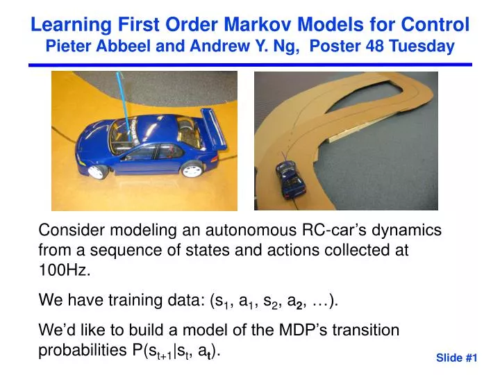
Learning First Order Markov Models for Control Pieter Abbeel and Andrew Y. Ng, Poster 48 Tuesday

1. Learning First Order Markov Models for ControlPieter Abbeel and Andrew Y. Ng, Poster 48 Tuesday • Consider modeling an autonomous RC-car’s dynamics from a sequence of states and actions collected at 100Hz. • We have training data: (s1, a1, s2, a2, …). • We’d like to build a model of the MDP’s transition probabilities P(st+1|st, at). Slide #1

2. Learning First Order Markov Models for ControlPieter Abbeel and Andrew Y. Ng, Poster 48 Tuesday • If we use maximum likelihood (ML) to fit the parameters of the MDP, then we are constrained to fit only the 1-step transitions: maxt p(st+1 | st, at) • But in RL, our goal is to maximize the long-term rewards, so we aren’t really interested in the 1/100th-second dynamics. • The dynamics on longer time-scales are often only poorly approximated (assuming the system isn’t really first-order). • Algorithms for building models that better capture dynamics on longer time-scales. • Experiments on autonomous RC car driving. Slide #2

3. Learning First Order Markov Models for Control Pieter Abbeel and Andrew Y. Ng Stanford University

4. Autonomous RC Car

5. Motivation • Consider modeling an RC-car’s dynamics from a sequence of states and actions collected at 100Hz. • Maximum likelihood fitting of a first order Markov model constrains the model to fit only the 1-step transitions. However for control applications, we do not care only about the dynamics on the time-scale of 1/100 of a second, but also about longer time-scales.

6. Motivation • If we use maximum likelihood (ML) to fit the parameters of a first-order Markov model, then we are constrained to fit only the 1-step transitions. • The dynamics on longer time-scales are often only poorly approximated [unless the system dynamics are really first-order]. • However for control: interested in maximizing the long-term expected rewards.

7. Random Walk Example • Random walk. • Consider two cases • Increments i independent: Var(ST) = T. • Increments i perfectly correlated: Var(ST) = T2. Regardless of true model, ML will return same model with .

8. Examples of physical systems • Influence of wind disturbances on helicopter • Very small over one time step. • Strong correlations lead to substantial effect over time. • Systematic model errors can show up as correlated noise. E.g., oversteering or understeering of car. • First order ML model may overestimate ability to control helicopter and car [thinking variance is O(T) rather than O(T2)]. This leads to danger of, e.g., flying too close to a building, or driving on too narrow a road.

9. Problem statement • The learning problem: • Given: state/action sequence data from a system. • Goal: model the system for purposes of control (such as to use with a RL algorithm). • Even when dynamics are not governed by an MDP, we often would still like to model it as such (rather than as a POMDP), since MDPs are much easier to solve. • How do we learn an accurate first order Markov model from data for control? [Our ideas are also applicable to higher order, and/or more structured models such as dynamic Bayesian networks and mixed memory Markov models.]

10. Preliminaries and Notation • Finite-state decision process (DP) • S: set of states, • A: set of actions, • P: set of state transition probabilities [not Markov!] • : discount factor, • D: initial state distribution, • R: reward function, 8s R(s) ·Rmax . • We will fit a model , with estimates of the transition probabilities . • Value of state s0 in under policy 

11. Parameter estimation when no actions • Consider Where is the variational distance. • dvar is hard to optimize from samples, but can be upper-bounded by a function of KL-divergence. • Minimizing KL-divergence is, in turn, identical to minimizing log-loss.

12. dvarKLlog-likelihood [The last step reflects we are equally interested in every state as possible starting state s0.]

13. The resulting lagged objective • Given a training sequence s0:T, we propose to use • Compare this to the maximum likelihood objective

14. Consider a length four training sequence, which could have various dependencies. S2 S2 S2 S2 S0 S0 S0 S0 S3 S3 S3 S3 S1 S1 S1 S1 Lagged objective vs. ML • ML takes into account only the following transitions: • Our lagged objective also takes into account: S1 S2 S2 S1 [Yellow nodes are observed, white nodes are unobserved.]

15. EM-algorithm to optimize lagged objective • E-step: compute expected counts and store in stats. I.e., 8t, k, l, i, j • M-step: update such that

16. Computational Savings for E-step • Inference for E-step can be done using standard forward and backward message passing. For every pair (t, t+k), the forward messages at position t+i depend on t only, not on k. So, computation of different terms in the inner-summation can share messages. Similarly for backward messages. This reduces the number of message computations by a factor T. • Often only interested in some maximum horizon H. I.e., in the inner-summation of the objective only consider k=1,…,H. Reduction from O(T3) to O(T H2). • More substantial savings: (St=i, St+k=j) and (St’=i, St’+k=j) contribute same to stats( . , . ) Computing stats( . , . ) contribution for all such pairs only once. Further reduction to O(|S|2 H2).

17. Incorporating actions • If actions are incorporated, our objective becomes: • The EM-algorithm is trivially extended by conditioning • on the actions during the E-step. • Forward messages need to be computed only once for • every t, backward messages once for every t+k. [as before] • Number of possibilities for at:t+k-1 is O(|A|k). • Use only a few deterministic exploration policies. •  Can still obtain same computational savings as before.

18. Experiment 1: shortest vs. safest path • Actions are 4 compass directions. • Move in intended direction with probability 0.7, and a random direction with probability 0.3. • The directions of the “random transitions” are dependent, and correlated over time. A parameter q controls the correlation between the directions of the random transitions on different time steps (uncorrelated if q=0, perfectly correlated if q=1). • We will fit a first order Markov model to these dynamics (with each grid position being a state). [Details: Noise process governed by a Markov process (not directly observable by the agent) with each of the 4 directions as states, with Prob(staying in same state) = q.]

19. Experiment 1: shortest vs. safest path (q) If the noise is strongly correlated across time (large q), our model estimates the dynamics to have a higher “effective noise level.” As a consequence the more cautious policy (path B) is used. [Details: Learning was done using a 200,000 length state-action sequence. Reported results are averages over 5 independent trials. The exploration policy used independent random actions at each time step.]

20. Experiment 2: Queue Customers arrive over time to be served. At every time, the arrival probability equals p. Service rate = probability that the customer first in queue gets serviced successfully in the current time step. • Actions: 3 service rates, with faster service rates being more expensive. • q0 = 0 reward = 0 • q1 = p reward = -1 • q2 = .75 reward = -10 • Queue buffer length = 20; buffer overflow results in reward -1000.

21. Experiment 2: Queue Underlying (unobserved!) arrival process has 2 different modes (fast arrivals and slow arrivals) • P( arrival | slow mode ) = 0.01 • P( arrival | fast mode ) = 0.99 • Steady state: P(slow mode)=0.8, P(fast mode)=0.2 Additional parameter determines how rapidly system changes between fast and slow modes. Slow switching between modes Fast switching between modes

22. Experiment 2: Queue Estimate/Learn first order Markov model with • State = size of the queue, Actions = 3 service rates • Exploration policy = repeatedly use same service rate for 25 time-steps. We used 8000 such trials. 15% better performance at high correlation levels. Same performance at low correlation levels.

23. Experiment 3: RC-car • Consider the situation where the RC-car can choose between 2 paths • A curvy path with high reward if successful in reaching the goal. • An easier path with lower reward if successful in reaching the goal • We build a dynamics model of the car, and find a policy/controller in simulation for following each of the paths. The decision about which path to follow is then made based upon this simulation.

24. RC-car model •  : angular direction the RC-car is headed •  : angular velocity • V : velocity of the RC-car (kept constant) • ut : steering input to the car ( 2 [-1,1]) • C1, C2, C3 : parameters of the model, estimated using linear regression • wt : noise term, zero-mean Gaussian with variance 2 . Using the lagged objective, we re-estimate the variance 2, and compare its performance to the first-order estimate of 2.

25. Controller • We use the following controller desired steering angle = p1*(y-ydes) + p2*(-des); u = f(desiredsteeringangle); We optimize over the parameters p1, p2 to follow the straight line y=0, for which we set ydes=0, des=0. For the specific two trajectories, ydes(x), des(x) are optimized as a function of the current x position. • For localization, we use an overhead camera.

26. Simulated performance on curvy trajectory Plot shows 100 sample runs in simulation under the ML-model. The ML-model predicts the RC-car can follow the curvy road >95% of the time. Plot shows 10 sample runs in simulation under the lag-learned model. The lag-learned model predicts the RC-car can follow the curvy road < 10% of the time. Green lines: simulated trajectories, Black lines: road boundaries.

27. Simulated performance on easier trajectory Plot shows 100 sample runs in simulation under the lag-learned model. The lag-learned model predicts the RC-car can follow the curvy road > 70% of the time. Plot shows 100 sample runs in simulation under the ML-model. The ML-model predicts the RC-car can follow the easier road >99% of the time.  ML would choose the curvy road if high reward along curvy road. Green lines: simulated trajectories, Black lines: road boundaries.

28. Actual performance on easier trajectory The real RC-car failed on the curvy road 19/20 times. The real RC-car succeeded on the easier road 20/20 times. [Movies available.]

29. RC-car movie

30. Conclusions • Maximum likelihood with a first order Markov model only tries to model the 1-step transition dynamics. • For many control applications, we desire an accurate model of the dynamics on longer time-scales. • We showed that, by using an objective that takes into account the longer time scales, in many cases a better dynamical model (and a better controller) is obtained. Special thanks to Mark Woodward, Dave Dostal, Vikash Gilja and Sebastian Thrun.

31. Cut out slides follow

32. Lagged objective vs. ML • Consider a length four training sequence, which could have various dependencies. • ML takes into account only the following transitions. • Our lagged objective also takes into account [Shaded nodes are observed, white nodes are unobserved.]

33. Experiment 2: Queue [use this one or previous one?] Queue size at time t+1 Queue size at time t unsuccessful servicing s(t+1) = s(t)+1 arrival successful servicing s(t) s(t+1) = s(t) unsuccessful servicing no arrival s(t+1) = s(t)-1 Arrival probability = p successful servicing • Choice of actions between 3 service rates • q0 = 0 reward = 0 • q1 = p reward = -1 • q2 = .75 reward = -10 • Buffer size = 20. Buffer overflow results in reward of -1000.

34. Actual performance on curvy trajectory Real trajectories obtained as obtained on floor. The actual RC-car fell off the curvy trajectory 19/20 times. [Movies available.] Green lines: simulated trajectories, Black lines: road boundaries.

35. Alternative title slides follow

36. Learning First Order Markov Models for Control Pieter Abbeel and Andrew Y. Ng Stanford University

37. Learning First

38. Order Markov

39. Models for

40. Control

41. Pieter Abbeel and Andrew Y. Ng Stanford University

42. Pieter Abbeel and Andrew Y. Ng Stanford University