Download
1 / 34
380 likes | 522 Views
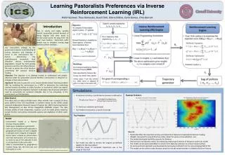
1. Algorithms for Inverse Reinforcement Learning 2. Apprenticeship learning via Inverse Reinforcement Learning. Algorithms for Inverse Reinforcement Learning Andrew Ng and Stuart Russell. Motivation.

E N D
1. Algorithms for Inverse Reinforcement Learning2. Apprenticeship learning via Inverse Reinforcement Learning
Algorithms for Inverse Reinforcement LearningAndrew Ng and Stuart Russell
Motivation • Given: (1) measurements of an agent's behavior over time, in a variety of circumstances, (2) if needed, measurements of the sensory inputs to that agent; (3) if available, a model of the environment. • Determine: the reward function being optimized.
Why? • Reason #1: Computational models for animal and human learning. • “In examining animal and human behavior we must consider the reward function as an unknown to be ascertained through empirical investigation.” • Particularly true of multiattribute reward functions (e.g. Bee foraging: amount of nectar vs. flight time vs. risk from wind/predators)
Why? • Reason #2: Agent construction. • “An agent designer [...] may only have a very rough idea of the reward function whose optimization would generate 'desirable' behavior.” • e.g. “Driving well” • Apprenticeship learning: Recovering expert's underlying reward function more “parsimonious” than learning expect's policy?
Possible applications in multi-agent systems • In multi-agent adversarial games, learning opponents’ reward functions that guild their actions to devise strategies against them. • example • In mechanism design, learning each agent’s reward function from histories to manipulate its actions. • and more?
Inverse Reinforcement Learning (1) – MDP Recap • MDP is represented as a tuple (S, A, {Psa}, ,R) Note: R is bounded by Rmax • Value function for policy : • Q-function:
Inverse Reinforcement Learning (1) – MDP Recap • Bellman Equation: • Bellman Optimality:
Inverse Reinforcement Learning (2)Finite State Space • Reward function solution set (a1 is optimal action)
Inverse Reinforcement Learning (2)Finite State Space There are many solutions of R that satisfy the inequality (e.g. R = 0), which one might be the best solution? 1. Make deviation from as costly as possible: 2. Make reward function as simple as possible
Va1 R? maximized Va2 Inverse Reinforcement Learning (2)Finite State Space • Linear Programming Formulation: a1, a2, …, an
Inverse Reinforcement Learning (3)Large State Space • Linear approximation of reward function (in driving example, basis functions can be collision, stay on right lane,…etc) • Let be value function of policy , when reward R = • For R to make optimal
Inverse Reinforcement Learning (3)Large State Spaces • In an infinite or large number of state space, it is usually not possible to check all constraints: • Choose a finite subset S0 from all states • Linear Programming formulation, find αi that: • x>=0, p(x)=x; otherwise p(x)=2x
Inverse Reinforcement Learning (4)IRL from Sample Trajectories • If is only accessible through a set of sampled trajectories (e.g. driving demo in 2nd paper) • Assume we start from a dummy state s0,(whose next state distribution is according to D). • In the case that reward trajectory state sequence (s0, s1, s2….):
Inverse Reinforcement Learning (4)IRL from Sample Trajectories • Assume we have some set of policies • Linear Programming formulation • The above optimization gives a new reward R, we then compute based on R, and add it to the set of policies • reiterate
Discrete Gridworld Experiment • 5x5 grid world • Agent starts in bottom-left square. • Reward of 1 in the upper-right square. • Actions = N,W,S,E (30% chance of random)
Mountain Car Experiment #1 • Car starts in valley, goal is at the top of hill • Reward is -1 per “step” until goal is reached • State = car's x-position & velocity (continuous!) • Function approx. class: all linear combinations of 26 evenly spaced Gaussian-shaped basis functions
Mountain Car Experiment #2 • Goal is in bottom of valley • Car starts... not sure. Top of hill? • Reward is 1 in the goal area, 0 elsewhere • γ = 0.99 • State = car's x-position & velocity (continuous!) • Function approx. class: all linear combinations of 26 evenly spaced Gaussian-shaped basis functions
Mountain Car Results #1 #2
Continuous Gridworld Experiment • State space is now [0,1] x [0,1] continuous grid • Actions: 0.2 movement in any direction + noise in x and y coordinates of [-0.1,0.1] • Reward 1 in region [0.8,1] x [0.8,1], 0 elsewhere • γ = 0.9 • Function approx. class: all linear combinations of a 15x15 array of 2-D Gaussian-shaped basis functions • m=5000 trajectories of 30 steps each per policy
Continuous Gridworld Results 3%-10% error when comparing fitted reward's optimal policy with the true optimal policy However, no significant difference in quality of policy (measured using true reward function)
Apprenticeship Learning via Inverse Reinforcement Learning Pieter Abbeel & Andrew Y. Ng
Algorithm • For t = 1,2,… • Inverse RL step: • Estimate expert’s reward function R(s)= wT(s) such that under R(s) the expert performs better than all previously found policies {i}. • RL step: • Compute optimal policy t for • the estimated reward w. Courtesy of Pieter Abbeel
Algorithm: IRL step • Maximize, w:||w||2≤ 1 • s.t. Vw(E) Vw(i) + i=1,…,t-1 • = margin of expert’s performance over the performance of previously found policies. • Vw() = E[t t R(st)|] = E[t t wT(st)|] • = wTE[t t (st)|] • = wT () • () = E[t t (st)|] are the “feature expectations” Courtesy of Pieter Abbeel
Feature Expectation Closeness and Performance • If we can find a policy such that • ||(E) - ()||2 , • then for any underlying reward R*(s) =w*T(s), • we have that • |Vw*(E) - Vw*()| = |w*T (E) - w*T ()| • ||w*||2 ||(E) - ()||2 • . Courtesy of Pieter Abbeel
|w*T (E) - w*T ()| = |Vw*(E) - Vw*()| = maximal difference between expert policy’s value function and 2nd to the optimal policy’s value function () IRL step as Support Vector Machine maximum margin hyperplane seperating two sets of points (E)
2 (E) (2) w(3) (1) w(2) w(1) Uw() = wT() (0) 1 Courtesy of Pieter Abbeel
Gridworld Experiment • 128 x 128 grid world divided into 64 regions, each of size 16 x 16 (“macrocells”). • A small number of macrocells have positive rewards. • For each macrocell, there is one feature Φi(s) indicating whether that state s is in macrocell i • Algorithm was also run on the subset of features Φi(s) that correspond to non-zero rewards.
Gridworld Results Distance to expert vs. # Iterations Performance vs. # Trajectories
Car Driving Experiment • No explict reward function at all! • Expert demonstrates proper policy via 2 min. of driving time on simulator (1200 data points). • 5 different “driver types” tried. • Features: which lane the car is in, distance to closest car in current lane. • Algorithm run for 30 iterations, policy hand-picked. • Movie Time! (Expert left, IRL right)